Chapter 01 — Schrödinger equation
The single most important equation in non-relativistic quantum mechanics. Every other equation in these notes is a special case, a mean-field approximation, or a comment on this one.
This chapter is the foundation under everything that follows. It does five things. (1) States the postulates that fix the formalism (section 1.2) and writes down the time-independent Schrödinger equation (TISE) for the electronic Hamiltonian in atomic units (section 1.1). (2) Walks through the particle in a box as a toy problem that lets us see the formalism in action, including a short Python finite-difference diagonalisation (section 1.3) and a catalogue of the operators that recur in every later chapter (section 1.4). (3) Derives the time-dependent Schrödinger equation (TDSE) from the time-dependent variational principle, reconstructs the TISE as the special case of a stationary state, and states the unitarity + continuity consequences (section 1.7). (4) Develops the operator formalism — linear operators on Hilbert space, the canonical commutation relations, the spectral theorem, and functions of operators such as the time-evolution operator $\hat U(t) = e^{-i\hat H t}$ (section 1.10) — and uses it to re-derive the time-evolution propagator, the stationary-state phase factor, and Fermi’s golden rule in operator language (section 1.11). (5) Closes the formal foundation with a preview of the symmetry and conservation-law structure of quantum mechanics (section 1.12): Noether’s theorem, the discrete symmetries of parity / time-reversal / particle–hole, and the selection rules they imply. The two exactly soluble many-body problems that anchor all of quantum chemistry are then solved within that framework: the harmonic oscillator (section 1.9) and the hydrogen atom (section 1.13). No prior quantum knowledge is assumed; every operator and every symbol is defined where it first appears.
Notation. We work throughout in atomic units ($\hbar = m_e = e = 4\pi\varepsilon_0 = 1$). Lengths are in Bohr ($a_0$), energies in Hartree ($E_h$). The conversion factors $1\,E_h \approx 27.211\,$eV and $1\,a_0 \approx 0.529\,$Å are used without comment when the answer needs to be quoted in laboratory units.
1.1 The time-independent Schrödinger equation
For a closed, non-relativistic, $N$-particle system with Hamiltonian $\hat H$, the stationary states $\psi$ and their energies $E$ are eigenpairs of $\hat H$:
\[\hat H \, \psi(\mathbf r_1, \dots, \mathbf r_N) = E \, \psi(\mathbf r_1, \dots, \mathbf r_N).\]For the rest of these notes we will almost always work with the electronic Hamiltonian in the Born–Oppenheimer (clamped-nuclei) approximation. In atomic units it reads
\[\hat H = -\frac{1}{2} \sum_{i=1}^{N} \nabla_i^2 \;-\; \sum_{i=1}^{N} \sum_{A=1}^{M} \frac{Z_A}{|\mathbf r_i - \mathbf R_A|} \;+\; \sum_{i<j}^{N} \frac{1}{|\mathbf r_i - \mathbf r_j|}.\]The three terms are, in order: the kinetic energy of the electrons, the electron–nuclear attraction, and the electron–electron repulsion. The nuclear–nuclear repulsion is a constant in the Born–Oppenheimer picture and is added at the end.
Tip. Many texts write the second term as $\sum_A Z_A / r_{iA}$ where $r_{iA} = \lvert \mathbf r_i - \mathbf R_A \rvert$. We will use the explicit vector form because it makes the gradient transparent when we derive the Kohn–Sham equations.
The TISE \eqref{eq:ch-01-tise} is the eigenvalue problem of quantum chemistry. Three of its features are worth pinning down before we move on.
- The spectrum is bounded from below. With $\hat H = \hat T + \hat V$ and the nuclear potential bounded, the kinetic term $\hat T = -\frac{1}{2}\sum_i \nabla_i^2$ is a positive semi-definite operator and the Coulomb singularity at $r_{ij} = 0$ is mild enough (it is integrable in 3-D) that $\hat H$ is bounded below. The lowest eigenvalue $E_0 \equiv \inf \sigma(\hat H)$ is the ground-state energy. The ground state is non-degenerate for atoms and molecules (Lions, 1987); excited states can be (and usually are) degenerate.
- Eigenfunctions form a complete orthonormal basis. The eigenfunctions ${\psi_n}$ of a self-adjoint operator on $L^2(\mathbb R^{3N})$ are complete in the sense that any square-integrable wavefunction has a convergent expansion $\Psi = \sum_n c_n \psi_n$ with $\sum_n |c_n|^2 < \infty$. This is the foundation of every expansion-based method in chapters 3, 5, 6.
- There is an inner product. $\langle \phi | \psi \rangle = \int \phi^(\mathbf x)\, \psi(\mathbf x)\, d\mathbf x$. The normalisation $\langle \psi | \psi \rangle = 1$ is *not built into $\hat H \psi = E \psi$; we impose it by hand and then keep it under unitary time evolution (section 1.7).
1.2 The postulates
The Schrödinger equation is postulated; the constants in it are measured; the rest is derived. We will use the Dirac–von Neumann axiomatisation:
| # | Postulate | Mathematical statement |
|---|---|---|
| P1 | States are rays in a Hilbert space | $\psi \in \mathcal H$, with $\lVert \psi \rVert = 1$ |
| P2 | Observables are self-adjoint operators | $\hat A : \mathcal H \to \mathcal H$, $\hat A = \hat A^\dagger$ |
| P3 | Measurements give eigenvalues | $\Pr(a_n) = \lvert \langle a_n \rvert \psi \rangle \rvert^2$ |
| P4 | Expectation values | $\langle A \rangle = \langle \psi \rvert \hat A \rvert \psi \rangle$ |
| P5 | Time evolution | $i \partial_t \lvert \psi(t) \rangle = \hat H \lvert \psi(t) \rangle$ |
| P6 | Indistinguishability | For identical fermions, $\Psi$ is totally antisymmetric under particle exchange |
P6 is the postulate that does almost all of the work in chemistry. It is also the postulate that DFT tries to circumvent.
A few words on each.
- P1. “States are rays” means that the global phase of $\psi$ carries no physics. The map $\psi \mapsto e^{i\alpha}\psi$ ($\alpha \in \mathbb R$) is a ray in the Hilbert space $\mathcal H$. The relative phase between two basis states, however, is physical (interference experiments see it), and the inner product structure of $\mathcal H$ is what tracks it.
- P2. Self-adjointness ($\hat A^\dagger = \hat A$) is the operator-level statement of “real eigenvalues for real measurements”. On a finite-dimensional subspace it reduces to Hermiticity; on the infinite-dimensional $L^2$ of continuous wavefunctions, the domain of $\hat A$ matters and self-adjointness is a non-trivial condition (it is not automatic, e.g. the momentum operator $i \partial_x$ is symmetric but not self-adjoint on $C_0^\infty(\mathbb R)$; its self-adjoint extension is on the Sobolev space $H^1(\mathbb R)$).
- P3, P4. Born’s rule: the squared modulus $|\langle a_n | \psi\rangle|^2$ is the probability of measuring $a_n$. The expectation value $\langle \psi | \hat A | \psi \rangle = \sum_n a_n |c_n|^2$ is the long-run average of those measurements.
- P5. The TDSE. It is linear in $|\psi\rangle$ (superposition is preserved) and unitary (probability is preserved, see section 1.7).
- P6. Indistinguishability. Exchange of two identical fermions multiplies the wavefunction by $-1$; for bosons, by $+1$. For electrons (spin-1/2 fermions) this is the mathematical content of the Pauli exclusion principle: two electrons cannot occupy the same spin-orbital, because the antisymmetrised product of two identical spin-orbitals is identically zero.
1.2.1 Mermaid — the postulates as a dependency graph
The six postulates are not independent: states (P1) are what observables (P2) act on, measurements (P3) and expectation values (P4) are statistics of the same object, time evolution (P5) is the dynamical law for that object, and the Pauli principle (P6) is the extra constraint that makes chemistry non-trivial. The diagram below makes those dependencies explicit.
graph TD
  subgraph foundations["Foundations"]
    P1["P1 — States<br/>|ψ⟩ ∈ ℋ, ||ψ|| = 1<br/>(ray in Hilbert space)"]
    P2["P2 — Observables<br/> = †<br/>(self-adjoint operator)"]
  end

  subgraph statics["Statics (TISE)"]
    P3["P3 — Measurement<br/>Pr(aₙ) = |⟨aₙ|ψ⟩|²"]
    P4["P4 — Expectation<br/>⟨Â⟩ = ⟨ψ|Â|ψ⟩"]
  end

  subgraph dynamics["Dynamics (TDSE)"]
    P5["P5 — Evolution<br/>i ∂ₜ|ψ⟩ = Ĥ|ψ⟩"]
  end

  subgraph symmetry["Symmetry"]
    P6["P6 — Antisymmetry<br/>Ψ(…, xᵢ, …, xⱼ, …) = −Ψ(…, xⱼ, …, xᵢ, …)"]
  end

  P1 --> P3
  P1 --> P4
  P2 --> P3
  P2 --> P4
  P1 --> P5
  P5 -->|"stationary limit<br/>(separation of vars)"| P3
  P3 --> P4
  P4 --> P5
  P6 -.->|"P1: antisymmetrised<br/>Slater determinants"| P1
  P6 -.->|"P5: phase-free,<br/>conserves norm"| P5
The solid arrows are “is-used-by”; the dashed arrows are “constrains”. P1–P5 are the kinematic postulates (they apply to any quantum system); P6 is the symmetry postulate and is what makes electronic-structure theory distinct from the quantum mechanics of distinguishable particles.
1.3 A minimal example: the particle in a box
To make the formalism concrete, consider a single electron in a 1-D box of length $L$ with infinite walls at $x = 0$ and $x = L$. The Hamiltonian is
\[\hat H = -\frac{1}{2}\,\frac{d^2}{dx^2}, \qquad \psi(0) = \psi(L) = 0.\]The normalised eigenfunctions and eigenvalues are
\[\psi_n(x) = \sqrt{\frac{2}{L}} \sin\!\left( \frac{n\pi x}{L} \right), \qquad E_n = \frac{\pi^2 n^2}{2 L^2}, \qquad n = 1, 2, 3, \dots\]A short Python snippet that solves the same problem numerically by
discretising the Laplacian and calling numpy.linalg.eigh:
# dft_notes/python_codes/chapter_01/01-particle-in-box.py
import numpy as np

def particle_in_a_box(L=1.0, N=400):
    """Return the first 5 eigenpairs of a 1-D particle in a box of length L."""
    h   = L / (N + 1)           # grid spacing
    x   = np.linspace(h, L - h, N)
    # 3-point stencil for the second derivative
    diag_main  = np.full(N,  2.0)
    diag_off   = np.full(N - 1, -1.0)
    H          = (np.diag(diag_main) + np.diag(diag_off, +1)
                                  + np.diag(diag_off, -1)) / (2 * h*`2)
    evals, evecs = np.linalg.eigh(H)
    # Sort by absolute value; skip the trivial infinite-wall mode
    order       = np.argsort(evals)
    return evals[order[:5]], evecs[:, order[:5]], x

energies, _, x = particle_in_a_box()
for n, E in enumerate(energies, start=1):
    exact = (np.pi * n)**2 / 2
    print(f"  n={n}  numerical={E:9.5f}  exact={exact:9.5f}  Δ={E - exact:+.2e}")
For a 400-point grid, the first five eigenvalues agree with the analytical formula to better than $10^{-8}$ Hartree.
Warning. A diagonalising eigensolver is never the right way to solve a real quantum chemistry problem — it costs $O(N^3)$ and stores $O(N^2)$. The point of the snippet is to make the formal eigenproblem $\hat H \psi = E \psi$ feel concrete. Production codes use iterative eigensolvers (Lanczos, Davidson) that never materialise the full Hamiltonian.
Connection to the time-dependent problem
The eigenstates of $\hat H$ form a stationary basis: if $|\psi(t)\rangle$ is a single eigenstate $|\psi_n\rangle$, then the TDSE $i \partial_t |\psi\rangle = \hat H |\psi\rangle$ gives
\[i \partial_t |\psi_n\rangle \;=\; E_n |\psi_n\rangle \;\;\Longrightarrow\;\; |\psi_n(t)\rangle \;=\; e^{-i E_n t} |\psi_n(0)\rangle .\]A superposition $|\psi(t)\rangle = \sum_n c_n e^{-i E_n t} |\psi_n\rangle$ acquires a time-dependent relative phase $e^{-i(E_n - E_m)t}$, which is what makes time evolution non-trivial. The probability density $|\psi(x,t)|^2$ is time-independent only for a single eigenstate or a degenerate superposition.
Visualisation — the first four eigenstates, animated
The static plot above is the end-state of the calculation. The animation below shows how the four wavefunctions appear one after the other, with a “particle” marker that traces the spatial oscillation; then a summary panel with the energy spectrum and the square moduli $|\psi_n|^2$.
1.4 Operators you will see again
The following operators are the alphabet of electronic-structure theory. They are all self-adjoint on the appropriate domain, which is why they are candidates for observables.
| Symbol | Name | Definition | Appears in |
|---|---|---|---|
| $\hat T$ | Kinetic energy | $\hat T = -\frac{1}{2} \sum_i \nabla_i^2$ | Every Hamiltonian |
| $\hat V_\text{ext}$ | External potential | $\hat V_\text{ext} = \sum_i v(\mathbf r_i)$ | The $Z_A / r_{iA}$ term |
| $\hat U_{ee}$ | Electron–electron repulsion | $\hat U_{ee} = \sum_{i<j} 1/r_{ij}$ | The $1/r_{ij}$ term |
| $\hat J$ | Classical Coulomb (Hartree) | $\hat J[\rho] = \int \rho(\mathbf r’) / \lvert \mathbf r - \mathbf r’ \rvert d\mathbf r’$ | Hartree–Fock, KS |
| $\hat K$ | Exchange (Fock) | $\hat K_{ij} = \int \phi_i^*(\mathbf r’) \phi_j(\mathbf r’) / \lvert \mathbf r - \mathbf r’ \rvert d\mathbf r’$ | Hartree–Fock |
| $\hat v_\text{xc}$ | XC potential | The functional derivative of $E_\text{xc}[\rho]$ with respect to $\rho$ | Kohn–Sham DFT |
| $\hat P_{ij}$ | Permutation | Exchanges particle labels $i \leftrightarrow j$ | Antisymmetrisation |
Two operators are so important they deserve a separate box.
Position and momentum. In atomic units, $\hat{\mathbf r}i = \mathbf r_i$ (multiplication) and $\hat{\mathbf p}_i = -i \nabla_i$. They satisfy the canonical commutation relation $[\hat r{ia}, \hat p_{jb}] = i \delta_{ij} \delta_{ab}$ for $a, b \in {x, y, z}$. This commutator is the defining algebraic structure of quantum mechanics; the Heisenberg uncertainty principle $\Delta A \Delta B \ge \frac{1}{2}|\langle [\hat A, \hat B] \rangle|$ is a direct consequence.
1.5 What we are not doing
Two things the Schrödinger equation does not give us, and that we have to add by hand or by approximation:
- Spin. The Hamiltonian above is spin-free. Spin enters via the antisymmetry postulate (P6) — electrons are fermions — and via the choice of $\Psi$ as a Slater determinant.
- Relativistic effects. For $Z \gtrsim 30$, the kinetic-energy term $-\frac{1}{2} \nabla^2$ should be replaced by the Dirac kinetic operator. Out of scope here; see a relativistic-chemistry text.
1.6 Outlook
The exact Schrödinger equation for a molecule with more than two or three electrons is unsolvable in closed form, and is intractable numerically because the wavefunction lives in a space whose dimension grows exponentially with $N$. The rest of these notes is a tour of the successive approximations that make the problem tractable: mean-field theory, density-functional reformulation, and the zoo of exchange–correlation functionals.
This chapter anchors every later one with five exact results that follow from the postulates alone: the operator formalism (commutators, spectral theorem, time-evolution operator) of section 1.10, the Dyson series and Fermi’s golden rule for time-dependent perturbations (section 1.8), the time-dependent Schrödinger equation (section 1.7), the harmonic oscillator (section 1.9), and the hydrogen atom (section 1.13). All five are needed before we can say what DFT is approximating.
Next: chapter 02 — the many-body problem and why a single Slater determinant isn’t enough.
1.7 The time-dependent Schrödinger equation
This section upgrades the postulates of section 1.2 from “the Hamiltonian has eigenstates” to “the wavefunction moves under $\hat H$”. The upgrade is more than cosmetic: time-dependent problems are the natural setting for spectroscopy, for response theory, and for every propagation method in molecular dynamics.
1.7.1 The TDSE postulate, again
Postulate P5 reads
\[i \frac{\partial}{\partial t} \lvert \psi(t) \rangle \;=\; \hat H \lvert \psi(t) \rangle .\]The Hamiltonian is independent of time (we are in the closed-system setting), so the formal solution is the time-evolution operator
\[\lvert \psi(t) \rangle \;=\; \hat U(t) \lvert \psi(0) \rangle , \qquad \hat U(t) \;=\; e^{-i \hat H t} . \tag{1.7.1}\]Three algebraic properties of $\hat U(t)$ follow directly from $\hat H$ being self-adjoint ($\hat H = \hat H^\dagger$).
- $\hat U(t)$ is unitary: $\hat U^\dagger(t) = e^{+i \hat H^\dagger t} = e^{+i \hat H t} = \hat U(-t) = \hat U(t)^{-1}$. Therefore $\langle \psi(t) | \psi(t) \rangle = \langle \psi(0) | \psi(0) \rangle = 1$ — probability is preserved. This is P1’s normalisation in motion.
- $\hat U(t)$ is one-parameter group: $\hat U(t_1)\hat U(t_2) = \hat U(t_1 + t_2)$. Time evolution is deterministic and reversible; given $|\psi(t)\rangle$, the state at any other time is fixed.
- $\hat U(t)$ commutes with $\hat H$: if $|\psi(0)\rangle$ is an eigenstate of $\hat H$ with eigenvalue $E_n$, then $\hat U(t) |\psi_n\rangle = e^{-i E_n t} |\psi_n\rangle$, which is just the statement that stationary states are stationary densities (only a global phase accumulates).
1.7.2 Derivation from the time-dependent variational principle
Postulate P5 follows from a single principle: stationary action. We require that the physical state $|\psi(t)\rangle$ make the action
\[\mathcal S[\psi] \;=\; \int_{t_1}^{t_2} \mathcal L\big[\psi(t), \partial_t \psi(t)\big]\, dt \tag{1.7.2}\]stationary against arbitrary variations $|\delta \psi(t)\rangle$ vanishing at the endpoints. The Lagrangian is the Dirac–Frenkel (or McLachlan) Lagrangian
\[\mathcal L[\psi, \partial_t \psi] \;=\; \langle \psi(t) \rvert\, i \partial_t - \hat H \, \rvert \psi(t) \rangle . \tag{1.7.3}\]It is a functional on the projective Hilbert space of normalised states; the factor of $i$ is the only choice that keeps $\mathcal L$ real and the resulting Euler–Lagrange equation linear and conservative.
Take an infinitesimal variation $|\psi\rangle \to |\psi\rangle + |\delta \psi\rangle$ with $\langle \delta \psi | \psi \rangle = 0$. Expanding and integrating by parts in $t$ (the boundary term vanishes because $|\delta \psi\rangle = 0$ at the endpoints), the stationarity condition $\delta \mathcal S = 0$ for arbitrary $|\delta \psi\rangle$ gives the Euler–Lagrange equation
\[i \partial_t \lvert \psi(t) \rangle \;=\; \hat H \lvert \psi(t) \rangle , \tag{1.7.4}\]which is postulate P5. Conversely, if the TDSE holds then $\mathcal L$ is constant in time, equal to $\langle E \rangle$ for normalised states. The TDSE is therefore the unique dynamics that is consistent with stationary action and unitarity (preservation of the inner product).
Tip. The Dirac–Frenkel action is the working horse of every ab-initio molecular-dynamics method (Car–Parrinello, surface-hopping, MCTDH, exact factorisation). The time-dependent Kohn–Sham equations of chapter 5 are recovered by restricting $|\psi(t)\rangle$ to a single Slater determinant and varying over the orbital rotations.
1.7.3 Separation of variables — recovering the TISE
Write $|\psi(t)\rangle = f(t) |\phi\rangle$. Substituting into \eqref{eq:ch-01-tdse-EL} and dividing by $f(t)|\phi\rangle$, the left-hand side is a pure function of $t$ and the right-hand side is a pure operator on $|\phi\rangle$, so both must equal a constant $E$. The time part is $i \dot f = E f \Rightarrow f(t) = e^{-i E t} f(0)$; the spatial part is
\[\hat H |\phi\rangle = E |\phi\rangle , \tag{1.7.5}\]which is the time-independent Schrödinger equation (TISE). The general solution is a sum of stationary states with time-dependent phases,
\[\lvert \psi(t) \rangle \;=\; \sum_n c_n\, e^{-i E_n t}\, \lvert \phi_n \rangle , \qquad \sum_n |c_n|^2 = 1 , \tag{1.7.6}\]with the $c_n$ determined by the initial condition. Two observations: the energy of a stationary state is sharp, but the expectation value of any operator that does not commute with $\hat H$ is not stationary (because the relative phases $e^{-i(E_n - E_m)t}$ rotate); and $\partial_t \langle \psi | \psi \rangle = 0$ by direct computation — the local version of which is the continuity equation of the next subsection.
1.7.4 Probability current and continuity
For a single particle in a real scalar potential $V(\mathbf r)$, subtract $\psi^*$ times the TDSE from $\psi$ times its complex conjugate:
\[i \partial_t |\psi|^2 \;=\; -\tfrac{1}{2}\, \nabla \cdot \big( \psi^* \nabla \psi - \psi \nabla \psi^* \big) .\]The left-hand side is $i\, \partial_t \rho$. Define the probability current
\[\mathbf j(\mathbf r, t) \;=\; \frac{1}{2i} \big[ \psi^* \nabla \psi - \psi \nabla \psi^* \big] \;=\; \operatorname{Im}\big( \psi^ \nabla \psi \big) . \tag{1.7.7}\]Then
\[\partial_t \rho(\mathbf r, t) + \nabla \cdot \mathbf j(\mathbf r, t) \;=\; 0 , \tag{1.7.8}\]the continuity equation. Integrate over a volume $V$ bounded by a surface $\partial V$ and use the divergence theorem:
\[\frac{d}{dt} \int_V \rho\, d\mathbf r \;=\; -\oint_{\partial V} \mathbf j \cdot d\mathbf S .\]Probability is conserved locally: any decrease inside $V$ equals the flux through the boundary. In the limit $V = \mathbb R^3$ with $\mathbf j \to 0$ at infinity, $\int \rho\, d\mathbf r$ is strictly time-independent, reproducing $\partial_t \langle \psi | \psi \rangle = 0$.
1.7.5 The Ehrenfest theorem
The TDSE also gives the equations of motion for expectation values. For any operator $\hat A$ (possibly explicitly time-dependent), differentiating $\langle \hat A \rangle$ and using the TDSE twice gives the Ehrenfest theorem
\[\frac{d}{dt} \langle \hat A \rangle \;=\; -\frac{i}{\hbar} \langle [\hat A, \hat H] \rangle + \Big\langle \frac{\partial \hat A}{\partial t} \Big\rangle . \tag{1.7.9}\]In atomic units, $d \langle \hat A\rangle / dt = -i \langle [\hat A, \hat H]\rangle + \langle \partial_t \hat A\rangle$. For $\hat A = \hat{\mathbf r}$: $[\hat{\mathbf r}, \hat H] = i\, \hat{\mathbf p}$, so $d \langle \mathbf r \rangle / dt = \langle \mathbf p \rangle$. For $\hat A = \hat{\mathbf p}$: $[\hat{\mathbf p}, \hat H] = -i\, \nabla V$, so $d \langle \mathbf p \rangle / dt = -\langle \nabla V \rangle$. Together,
\[m\, \frac{d^2 \langle \mathbf r \rangle}{dt^2} \;=\; -\Big\langle \nabla V(\mathbf r) \Big\rangle , \tag{1.7.10}\]which is Newton’s second law for the wavepacket’s centroid (when the potential is slowly varying over the wavepacket’s extent). Ehrenfest’s theorem is the bridge between quantum and classical mechanics; it justifies classical-trajectory molecular dynamics in the heavy-particle limit.
1.7.6 Mermaid: time evolution and stationarity
graph TD
  H0["Initial state<br/>|ψ(0)⟩"] --> EX["Expand in eigenbasis of H<br/>|ψ(0)⟩ = Σ c_n |n⟩"]
  EX --> P1{"Single eigenstate?"}
  P1 -->|"yes"| ST["Stationary:<br/>|ψ(t)⟩ = e^(-iE_n t)|n⟩<br/>|ψ|² time-independent"]
  P1 -->|"no (superposition)"| DY["Dynamic:<br/>|ψ(t)⟩ = Σ c_n e^(-iE_n t)|n⟩<br/>relative phases rotate"]
  ST --> USE1["Used in: spectroscopy baselines,<br/>stationary perturbation theory"]
  DY --> USE2["Used in: TDDFT, wavepacket dynamics,<br/>Fermi's golden rule (1.8)"]
This is the conceptual flow for the rest of the chapter. The stationary branch recovers the TISE; the dynamic branch is the starting point for time-dependent perturbation theory.
1.8 Time-dependent perturbation theory
Most quantum systems of chemical interest cannot be solved exactly, but most can be written as a known, exactly soluble system plus a small perturbation. The Dyson series and Fermi’s golden rule are the formal apparatus that converts that intuition into numbers.
1.8.1 The interaction picture
The starting point is a Hamiltonian split into a bare (solvable) part and a perturbation,
\[\hat H(t) \;=\; \hat H_0 + \hat V(t) , \tag{1.8.1}\]where we will be interested in the case where $\hat V(t)$ is switched on smoothly from $t = -\infty$, $\hat V(t) = e^{\eta t} \hat V$ for $t \to -\infty$ with $\eta \to 0^+$, and constant for $t \ge 0$. The Dyson series works for any $\hat V(t)$; the smooth switching is the adiabatic switching that avoids the $\delta(0)$ divergences of sudden turn-on.
The interaction picture state is
\[\lvert \psi_I(t) \rangle \;=\; e^{i \hat H_0 t}\, \lvert \psi_S(t) \rangle , \tag{1.8.2}\]where the subscript $S$ denotes the Schrödinger picture. The Schrödinger evolution is $|\psi_S(t)\rangle = \hat U(t, t_0) |\psi_S(t_0)\rangle$ with $\hat U(t, t_0) = \mathcal T \exp!\big[-i \int_{t_0}^t \hat H(t’)\, dt’\big]$ (the time-ordered exponential, where $\mathcal T$ orders later times to the left). Inserting the definition of $|\psi_I\rangle$:
\[\lvert \psi_I(t) \rangle \;=\; e^{i \hat H_0 t} \hat U(t, t_0) e^{-i \hat H_0 t_0}\, \lvert \psi_I(t_0) \rangle \;\equiv\; \hat U_I(t, t_0)\, \lvert \psi_I(t_0) \rangle . \tag{1.8.3}\]Differentiate with respect to $t$ and use $i \partial_t \hat U = \hat H \hat U$ and $i \partial_t e^{i\hat H_0 t} = -\hat H_0 e^{i\hat H_0 t}$:
\[i \partial_t \lvert \psi_I(t) \rangle \;=\; e^{i \hat H_0 t}\, \hat V_I(t)\, e^{-i \hat H_0 t}\, \lvert \psi_I(t) \rangle ,\]where the interaction-picture perturbation operator is
\[\hat V_I(t) \;=\; e^{i \hat H_0 t}\, \hat V(t)\, e^{-i \hat H_0 t} . \tag{1.8.4}\]The interaction-picture evolution operator $\hat U_I(t, t_0)$ therefore satisfies
\[i \partial_t \hat U_I(t, t_0) \;=\; \hat V_I(t)\, \hat U_I(t, t_0) , \qquad \hat U_I(t_0, t_0) = \hat 1 . \tag{1.8.5}\]Equation \eqref{eq:ch-01-u-ido} is equivalent to the integral form
\[\hat U_I(t, t_0) \;=\; \hat 1 - i \int_{t_0}^t \hat V_I(t_1)\, \hat U_I(t_1, t_0)\, dt_1 . \tag{1.8.6}\]1.8.2 The Dyson series
Iterating \eqref{eq:ch-01-u-ido-integral} gives the Dyson series
\[\hat U_I(t, t_0) \;=\; \sum_{n=0}^{\infty} \frac{(-i)^n}{n!} \int_{t_0}^{t} \!\!\!\cdots\!\! \int_{t_0}^{t} \mathcal T\!\big[ \hat V_I(t_1) \hat V_I(t_2) \cdots \hat V_I(t_n) \big]\, dt_1 \cdots dt_n . \tag{1.8.7}\]The first two terms are obtained by iteration of \eqref{eq:ch-01-u-ido-integral}. At $n = 0$, $\hat U_I = \hat 1$. Substituting this into \eqref{eq:ch-01-u-ido-integral} gives the first Born approximation
\[\hat U_I(t, t_0) \;\approx\; \hat 1 - i \int_{t_0}^{t} \hat V_I(t_1)\, dt_1 + \mathcal O(\hat V^2) . \tag{1.8.8}\]Inserting \eqref{eq:ch-01-born1} back into \eqref{eq:ch-01-u-ido-integral} produces the $n = 2$ term; in symmetrised form,
\[\frac{(-i)^2}{2!} \int_{t_0}^{t} \!\! \int_{t_0}^{t} dt_1\, dt_2\, \mathcal T\!\big[ \hat V_I(t_1) \hat V_I(t_2) \big] \;=\; (-i)^2 \int_{t_0}^{t} dt_1 \int_{t_0}^{t_1} dt_2\, \hat V_I(t_1) \hat V_I(t_2) ,\]because $\mathcal T$ puts the later-time operator on the left and the $t_1 \ge t_2$ ordering restricts half the integration domain. Continuing the iteration to all orders gives \eqref{eq:ch-01-dyson}. The series is the perturbative expansion of the time-evolution operator in powers of $\hat V$; at $n$-th order, exactly $n$ factors of $\hat V_I$ appear, time-ordered left-to-right from earliest to latest.
1.8.3 First-order transition amplitude
The probability amplitude to transition from an initial eigenstate $|i\rangle$ of $\hat H_0$ to a final eigenstate $|f\rangle$ at time $t$ is, in first-order perturbation theory,
\[c_f^{(1)}(t) \;=\; \langle f \rvert \hat U_I(t, 0) \rvert i \rangle \;\approx\; -i \int_0^t \langle f \rvert \hat V_I(t_1) \rvert i \rangle\, dt_1 . \tag{1.8.9}\]Use \eqref{eq:ch-01-vint}: $\hat V_I(t) = e^{i \hat H_0 t} \hat V(t) e^{-i \hat H_0 t}$, so $\langle f | \hat V_I(t_1) | i \rangle = e^{i(E_f - E_i) t_1} V_{fi}(t_1)$, where $V_{fi}(t) \equiv \langle f | \hat V(t) | i \rangle$ is the matrix element of the perturbation in the $\hat H_0$ basis. Therefore
\[c_f^{(1)}(t) \;=\; -i \int_0^t e^{i \omega_{fi} t_1} V_{fi}(t_1)\, dt_1 , \qquad \omega_{fi} \equiv E_f - E_i . \tag{1.8.10}\]For a time-independent perturbation $\hat V$ (the most common case in spectroscopy and scattering), $V_{fi}$ is constant, and the integral is elementary:
\[c_f^{(1)}(t) \;=\; -i\, V_{fi}\, \int_0^t e^{i \omega_{fi} t_1}\, dt_1 \;=\; -i\, V_{fi}\, \frac{e^{i \omega_{fi} t} - 1}{i \omega_{fi}} \;=\; V_{fi}\, \frac{1 - e^{i \omega_{fi} t}}{\omega_{fi}} . \tag{1.8.11}\]The transition probability is the squared modulus,
\[P_{i \to f}(t) \;=\; |c_f^{(1)}(t)|^2 \;=\; |V_{fi}|^2\, \frac{4 \sin^2(\omega_{fi} t / 2)}{\omega_{fi}^2} \;=\; |V_{fi}|^2\, \frac{2 - 2\cos(\omega_{fi} t)}{\omega_{fi}^2} . \tag{1.8.12}\]For long times $t$, the function $2 \sin^2(\omega t/2)/\omega^2$ becomes concentrated around $\omega = 0$; this is the resonance condition $E_f = E_i$.
1.8.4 Fermi’s golden rule
We want the rate of transitions from $|i\rangle$ into a continuum of final states ${|f\rangle}$ of similar energy. Sum \eqref{eq:ch-01-prob1} over a band of final states with density of states $\rho_f(E_f)$ (in energy, not in state-index), and pass to the long-time limit:
\[\Gamma_{i \to f} \;=\; \lim_{t \to \infty} \frac{d}{dt} \sum_{f} P_{i \to f}(t) .\]Differentiating \eqref{eq:ch-01-prob1} and using $d/dt [2 - 2\cos(\omega t)] = 2 \omega \sin(\omega t)$,
\[\frac{d P_{i \to f}}{dt} \;=\; 2 |V_{fi}|^2\, \frac{\sin(\omega_{fi} t)}{\omega_{fi}} . \tag{1.8.13}\]Sum over $f$ by replacing the discrete sum with an integral over $E_f$ weighted by $\rho_f(E_f)$:
\[\sum_f \frac{d P_{i \to f}}{dt} \;=\; 2 \int |V_{fi}(E_f)|^2\, \rho_f(E_f)\, \frac{\sin(\omega_{fi} t)}{\omega_{fi}}\, dE_f .\]Use $\omega_{fi} = E_f - E_i$, so $dE_f = d\omega_{fi}$. The function $\sin(\omega t)/\omega$ is a nascent delta: it integrates to $\pi$ in the limit $t \to \infty$,
\[\int_{-\infty}^{\infty} \frac{\sin(\omega t)}{\omega}\, d\omega \;=\; \pi .\]In detail, it is the Dirac kernel
\[\delta_t(\omega) \;\equiv\; \frac{\sin(\omega t)}{\pi \omega} \;\;\xrightarrow{t \to \infty}\;\; \delta(\omega) . \tag{1.8.14}\]Replacing $\delta_t$ by $\delta$, the integral collapses to the value at the resonance $E_f = E_i$:
\[\sum_f \frac{d P_{i \to f}}{dt} \;\xrightarrow{t \to \infty}\; 2 \pi\, |V_{fi}(E_i)|^2\, \rho_f(E_i) .\]This is the transition rate, and the result is Fermi’s golden rule:
\[\boxed{ \Gamma_{i \to f} \;=\; \frac{2 \pi}{\hbar}\, |V_{fi}|^2\, \rho_f(E_f)\Big|_{E_f = E_i} } \tag{1.8.15}\](in atomic units, $\hbar = 1$, and the prefactor is just $2\pi$). Equation \eqref{eq:ch-01-fermi} is the workhorse of spectroscopy: the rate of an $|i\rangle \to |f\rangle$ transition is the square of the matrix element of the perturbation between the two states, times the density of final states at the resonance energy. We will use it in section 1.13 to compute the spontaneous-emission rate of the hydrogen $2p \to 1s$ transition.
Tip. Fermi’s golden rule is first order in the perturbation but all orders in $\hat H_0$. It is exact in the limit of a small, time-independent perturbation, no matter how complicated $\hat H_0$ is. The price of this generality is that the line shape (a Lorentzian of width $\Gamma$ in practice) is determined by the imaginary part of the self-energy and is not captured at first order; for that, one uses the second-order self-energy (Fermi–Wigner–Weisskopf line shape) or the resolvent approach of Heitler–Ma.
1.8.5 Mermaid: time-dependent perturbative expansion
graph LR
  subgraph "Order-by-order wavefunction evolution"
    direction LR
    P0["|ψ⁽⁰⁾(t)⟩<br/>e^(-iE_i t)|i⟩"] --> P1["|ψ⁽¹⁾(t)⟩<br/>+ ∫_0^t e^(-iH₀(t-t₁)) V |i⟩ dt₁"]
    P1 --> P2["|ψ⁽²⁾(t)⟩<br/>+ ∫∫ e^(-iH₀(t-t₁)) V e^(-iH₀(t₁-t₂)) V |i⟩ dt₁dt₂"]
    P2 --> P3["|ψ⁽ⁿ⁾(t)⟩<br/>n nested commutators"]
  end
  P1 --> AMP["Amplitude c_f^(n)(t)<br/>= ⟨f|ψ⁽ⁿ⁾(t)⟩"]
  P2 --> AMP
  P3 --> AMP
  AMP --> RATE["|c_f|² → rate<br/>Fermi's golden rule<br/>(long-time, resonance)"]
Each “order” in the expansion adds one more factor of $\hat V$ and one more time integral. The first-order amplitude gives the leading transition rate, Fermi’s golden rule.
1.9 The harmonic oscillator
The quantum harmonic oscillator (QHO) is the most important exactly soluble problem in quantum mechanics. It describes molecular vibrations in the harmonic approximation, the phonons of a crystal, the normal modes of a transition state, and — in second quantisation — every bosonic field. We solve it twice: algebraically (ladder operators) and in position space (Hermite polynomials).
1.9.1 The Hamiltonian
For a particle of mass $m$ and angular frequency $\omega$ in a 1-D harmonic well, the Hamiltonian is
\[\hat H \;=\; \frac{\hat p^2}{2m} + \frac{1}{2} m \omega^2 \hat x^2 . \tag{1.9.1}\]In atomic units, $m = 1$ for the electron, and the kinetic term is $-\tfrac{1}{2} \partial_x^2$. The characteristic length and energy scales are
\[x_0 \;=\; \frac{1}{\sqrt{m\omega}}, \qquad E_0 \;=\; \frac{\omega}{2} . \tag{1.9.2}\]Define the dimensionless position $\hat q = \hat x / x_0$ and dimensionless momentum $\hat p’ = x_0\, \hat p$, which satisfy $[\hat q, \hat p’] = i$. The Hamiltonian in dimensionless units is
\[\hat H \;=\; \frac{\omega}{2}\, \big( \hat p'^2 + \hat q^2 \big) . \tag{1.9.3}\]Drop the primes; everything below is in dimensionless units. The position-space form is
\[\hat H \;=\; -\frac{\omega}{2}\, \frac{d^2}{dq^2} + \frac{\omega}{2}\, q^2 . \tag{1.9.4}\]1.9.2 Ladder operators
Define the annihilation and creation operators
\[\hat a \;=\; \frac{1}{\sqrt{2}}\big( \hat q + i \hat p \big) , \qquad \hat a^\dagger \;=\; \frac{1}{\sqrt{2}}\big( \hat q - i \hat p \big) . \tag{1.9.5}\]Their commutation relation follows from $[\hat q, \hat p] = i$:
\[[\hat a, \hat a^\dagger] \;=\; \frac{1}{2} \big[ \hat q + i\hat p,\, \hat q - i\hat p \big] \;=\; \frac{1}{2} \big( -i [\hat q, \hat p] + i [\hat p, \hat q] \big) \;=\; \frac{1}{2}\, ( -i\, i + i\, (-i) ) \;=\; 1 . \tag{1.9.6}\]So $[\hat a, \hat a^\dagger] = \hat 1$ (the bosonic CCR). The Hamiltonian \eqref{eq:ch-01-qho-h-dim} is, inverting \eqref{eq:ch-01-ladd-def},
\[\hat q \;=\; \frac{1}{\sqrt{2}} \big( \hat a + \hat a^\dagger \big) , \qquad \hat p \;=\; \frac{i}{\sqrt{2}} \big( \hat a^\dagger - \hat a \big) ,\]and therefore
\[\hat q^2 + \hat p^2 \;=\; \tfrac{1}{2}(\hat a + \hat a^\dagger)^2 - \tfrac{1}{2}(\hat a^\dagger - \hat a)^2 \;=\; \hat a \hat a^\dagger + \hat a^\dagger \hat a .\]Substituting,
\[\hat H \;=\; \frac{\omega}{2}\, \big( \hat a \hat a^\dagger + \hat a^\dagger \hat a \big) \;=\; \omega \big( \hat a^\dagger \hat a + \tfrac{1}{2} \big) . \tag{1.9.7}\]The combination $\hat a^\dagger \hat a \equiv \hat n$ is the number operator; its eigenvalues are non-negative integers (we will see this in a moment), and the spectrum of $\hat H$ is therefore
\[E_n \;=\; \omega \big( n + \tfrac{1}{2} \big) , \qquad n = 0, 1, 2, \dots \tag{1.9.8}\]The ground-state energy $E_0 = \omega/2$ is the zero-point energy; it is non-zero because the Heisenberg uncertainty principle forbids a state with $\Delta x = \Delta p = 0$.
1.9.3 The energy spectrum from commutation
The spectrum \eqref{eq:ch-01-qho-spectrum} is fixed by the commutation relations alone, not by any differential-equation machinery. Compute
\[[\hat H, \hat a] \;=\; \omega [\hat a^\dagger \hat a, \hat a] \;=\; \omega \big( \hat a^\dagger [\hat a, \hat a] + [\hat a^\dagger, \hat a] \hat a \big) \;=\; -\omega \hat a . \tag{1.9.9}\]Therefore, if $|n\rangle$ is an eigenstate of $\hat H$ with eigenvalue $E_n$,
\[\hat H\, \hat a |n\rangle \;=\; \big( \hat a \hat H + [\hat H, \hat a] \big) |n\rangle \;=\; \big( E_n - \omega \big) \hat a |n\rangle . \tag{1.9.10}\]$\hat a |n\rangle$ is an eigenstate with eigenvalue $E_n - \omega$. Similarly $\hat a^\dagger |n\rangle$ is an eigenstate with eigenvalue $E_n + \omega$. The ladder of states is therefore
\[\cdots \;\xleftarrow{\hat a}\; |n\rangle \;\xrightarrow{\hat a^\dagger}\; |n+1\rangle ,\]and the energy spacing between adjacent levels is exactly $\omega$. (This is why a classical oscillator, Fourier-analysed, emits/absorbs energy in quanta of $\hbar \omega$.)
To pin down the absolute energy scale, the lowest-weight state $|0\rangle$ must be annihilated by $\hat a$: $\hat a |0\rangle = 0$. If it were not, $\hat a |0\rangle$ would be an eigenstate of $\hat H$ with eigenvalue $E_0 - \omega$, and iterating would give an unbounded-below spectrum (in contradiction to $\hat H$ being bounded below). So $\hat a |0\rangle = 0$ and $E_0 = \omega \langle 0|\hat a^\dagger \hat a|0\rangle + \omega/2 = \omega/2$. The rest of the spectrum follows from $|n\rangle = (n!)^{-1/2} (\hat a^\dagger)^n |0\rangle$, with $E_n = (n + 1/2)\omega$ and orthonormality $\langle m | n \rangle = \delta_{mn}$.
1.9.4 Position-space wavefunctions and Hermite polynomials
The position-space eigenfunctions are obtained from $\langle q | 0 \rangle \equiv \phi_0(q)$ by solving $\hat a \phi_0(q) = 0$, i.e. $\frac{1}{\sqrt 2}(q + d/dq) \phi_0(q) = 0$. The solution is a normalised Gaussian,
\[\phi_0(q) \;=\; \pi^{-1/4}\, e^{-q^2/2} . \tag{1.9.11}\]Excited states are generated by $\phi_n(q) = (n!)^{-1/2} (a^\dagger)^n \phi_0(q)$. In position space, the creation operator is $\hat a^\dagger = (q - d/dq)/\sqrt 2$, so $\hat a^\dagger \phi_n$ is a first-order differential operator acting on $\phi_n$. Iterating gives
\[\phi_n(q) \;=\; \frac{1}{\sqrt{2^n n!}}\, H_n(q)\, \pi^{-1/4}\, e^{-q^2/2} , \tag{1.9.12}\]where $H_n$ is the physicists’ Hermite polynomial, defined by
\[H_n(q) \;=\; (-1)^n e^{q^2}\, \frac{d^n}{dq^n}\, e^{-q^2} . \tag{1.9.13}\]The first few are $H_0 = 1$, $H_1 = 2q$, $H_2 = 4q^2 - 2$, $H_3 = 8q^3 - 12q$. The wavefunctions $\phi_n(q)$ are real, alternate in parity ($\phi_n(-q) = (-1)^n \phi_n(q)$), and have exactly $n$ zeros on the real line. In dimensionful variables the eigenfunctions are
\[\psi_n(x) \;=\; \frac{1}{\sqrt{x_0}}\, \phi_n\!\left( \frac{x}{x_0} \right) \;=\; \frac{1}{\sqrt{2^n n! \pi^{1/2} x_0}}\, H_n\!\left( \frac{x}{x_0} \right)\, \exp\!\left( -\frac{x^2}{2 x_0^2} \right) . \tag{1.9.14}\]1.9.5 Coherent states
A coherent state $|\alpha\rangle$ ($\alpha \in \mathbb C$) is an eigenstate of the annihilation operator,
\[\hat a \lvert \alpha \rangle \;=\; \alpha \lvert \alpha \rangle . \tag{1.9.15}\]It is the most classical state allowed by quantum mechanics: it minimises the Heisenberg uncertainty product $\Delta x \Delta p = 1/2$ (see Problem 3), it does not spread under free evolution, and its time evolution is $|\alpha(t)\rangle = |\alpha e^{-i\omega t}\rangle$ — a classical orbit in the $(\operatorname{Re}\alpha, \operatorname{Im}\alpha)$ phase plane.
The coherent state can be expanded in the Fock basis ${|n\rangle}$ as
\[\lvert \alpha \rangle \;=\; e^{-|\alpha|^2/2} \sum_{n=0}^{\infty} \frac{\alpha^n}{\sqrt{n!}}\, \lvert n \rangle . \tag{1.9.16}\]The probabilities are Poissonian, $P_n = |\langle n | \alpha \rangle|^2 = e^{-|\alpha|^2} |\alpha|^{2n} / n!$, with mean photon number $\langle \hat n \rangle = |\alpha|^2$. The position-space wavefunction is a displaced Gaussian,
\[\langle q | \alpha \rangle \;=\; \pi^{-1/4}\, \exp\!\Big[ -\tfrac{1}{2}(q - q_0)^2 + i p_0 (q - q_0/2) \Big] , \tag{1.9.17}\]where $q_0 = \sqrt 2 \operatorname{Re}\alpha$ and $p_0 = \sqrt 2 \operatorname{Im}\alpha$. Under free evolution ($H = \omega a^\dagger a$), the centre $(q_0(t), p_0(t))$ orbits the classical ellipse in $(q, p)$ space, exactly as a classical harmonic oscillator would.
The overcompleteness relation is
\[\frac{1}{\pi} \int \lvert \alpha \rangle \langle \alpha \rvert\, d^2\alpha \;=\; \hat 1 , \tag{1.9.18}\]so the coherent states resolve the identity despite not being orthogonal: $\langle \alpha | \beta \rangle = e^{-(|\alpha|^2 + |\beta|^2)/2 + \alpha^* \beta}$.
1.9.6 Mermaid: ladder-operator action and coherent states
graph LR
  subgraph "Ladder operators"
    G["|0⟩<br/>E = ω/2"] -->|"â†"| N1["|1⟩<br/>E = 3ω/2"]
    N1 -->|"â†"| N2["|2⟩<br/>E = 5ω/2"]
    N2 -->|"â†"| N3["|3⟩<br/>E = 7ω/2"]
    N3 --> D["…"]
  end

  G -.->|"â = 0"| GHOST["vacuum<br/>lowest-weight<br/>state"]
  N1 -.->|"â reduces n"| G
  N2 -.->|"â reduces n"| N1
  N3 -.->|"â reduces n"| N2
The QHO’s entire spectrum is generated by repeated application of $\hat a^\dagger$ to the vacuum $|0\rangle$, with $\hat a^\dagger \hat a$ acting as the “energy counter”.
graph TD
  C["Coherent state |α⟩<br/>eigenstate of â<br/>â|α⟩ = α|α⟩"] --> P1["Minimises Δx Δp<br/>(uncertainty product)"]
  C --> P2["P_n = e^(-N) N^n/n!<br/>Poisson statistics"]
  C --> P3["Free evolution =<br/>orbit in phase space<br/>|α(t)⟩ = |α e^(-iωt)⟩"]
  C --> P4["Resolves the identity:<br/>(1/π)∫ |α⟩⟨α| d²α = 1̂"]
1.10 Operator formalism
Sections 1.7–1.9 used operators freely — the Hamiltonian, the position and momentum operators, the annihilation and creation operators — but treated them as the objects of differential equations. This section lifts that treatment to the abstract operator level: definitions that do not depend on a particular representation, properties of operators under addition and multiplication, and the key commutator structure that makes quantum mechanics what it is.
1.10.1 Linear operators on Hilbert space
A linear operator on the Hilbert space $\mathcal H$ is a map $\hat A: \mathcal H \to \mathcal H$ that preserves linear combinations,
\[\hat A \big( \alpha \lvert \psi \rangle + \beta \lvert \phi \rangle \big) \;=\; \alpha\, \hat A \lvert \psi \rangle + \beta\, \hat A \lvert \phi \rangle . \label{eq:ch-01-10-linear} \tag{1.10.1}\]Every operator used in the rest of these notes is linear. The adjoint (or Hermitian conjugate) $\hat A^\dagger$ of a linear operator is defined by
\[\langle \phi \rvert \hat A \psi \rangle \;=\; \langle \hat A^\dagger \phi \rvert \psi \rangle \qquad \text{for all } \lvert \phi \rangle, \lvert \psi \rangle \in \mathcal H . \label{eq:ch-01-10-adjoint} \tag{1.10.2}\]The adjoint reverses the order of products, $(\hat A \hat B)^\dagger = \hat B^\dagger \hat A^\dagger$, and maps scalars to their complex conjugates, $(\alpha \hat A)^\dagger = \alpha^* \hat A^\dagger$. Three special cases are worth singling out.
- Hermitian (self-adjoint) operators satisfy $\hat A^\dagger = \hat A$. They are the candidates for observables (postulate P2): their eigenvalues are real, and their eigenstates at distinct eigenvalues are orthogonal. All operators in section 1.4 (kinetic, potential, Coulomb, exchange, …) are Hermitian.
- Unitary operators satisfy
They preserve inner products ($\langle \hat U \psi \rvert \hat U \phi \rangle = \langle \psi \rvert \phi \rangle$) and norms, and are the candidates for symmetry operations (translations, rotations, time evolution). The time-evolution operator of section 1.11 is the most important unitary operator in these notes.
- Antiunitary operators satisfy $\hat A^\dagger \hat A = \hat 1$ but additionally take the complex conjugate of scalars, $\hat A (\alpha \lvert \psi \rangle) = \alpha^* \hat A \lvert \psi \rangle$. The time-reversal operator of section 1.12.2 is the only antiunitarian we will meet.
Tip. The bra-ket notation makes the adjoint operation easy: $\hat A^\dagger$ is the unique operator such that $\hat A^\dagger \lvert \phi \rangle$ is the bra $\langle \phi \rvert \hat A$. This is also why bras and kets come paired: a bra is the adjoint of a ket, and applying an operator to a ket is the same as premultiplying the corresponding bra by the adjoint.
1.10.2 Commutators and the canonical commutation relations
The commutator of two operators is
\[[\hat A, \hat B] \;=\; \hat A \hat B - \hat B \hat A . \label{eq:ch-01-10-commutator} \tag{1.10.4}\]Two operators commute if their commutator is zero; in that case they can be simultaneously diagonalised, and every eigenstate of one is an eigenstate of the other. The non-commutativity of operators is the distinguishing feature of quantum mechanics: it is what makes the uncertainty principle possible (see Problem 1), and it is the reason that position and momentum cannot both be sharp.
The commutation relations that define non-relativistic quantum mechanics are the canonical commutation relations (CCR),
\[[\hat x_a, \hat p_b] \;=\; i \delta_{ab} , \qquad [\hat x_a, \hat x_b] = [\hat p_a, \hat p_b] = 0 , \label{eq:ch-01-10-ccr} \tag{1.10.5}\]where $a, b \in {x, y, z}$. (We work in atomic units, so $\hbar = 1$ is implicit; the SI form is $[\hat x_a, \hat p_b] = i\hbar \delta_{ab}$.) The multi-particle generalisation is $[\hat r_{ia}, \hat p_{jb}] = i \delta_{ij} \delta_{ab}$ for $i, j \in {1, \dots, N}$. The CCR is not derived from anything more fundamental; it is the defining algebraic structure of quantum mechanics, and every other commutation relation in these notes — angular-momentum algebra, fermionic and bosonic commutation rules, the Lie algebra of the Lorentz group — is built on top of it.
Two operator identities are used so often that we name them now. The Leibniz rule for commutators,
\[[\hat A, \hat B \hat C] \;=\; [\hat A, \hat B]\, \hat C + \hat B\, [\hat A, \hat C] , \label{eq:ch-01-10-leibniz} \tag{1.10.6}\]and its analogue for the anticommutator ${\hat A, \hat B} = \hat A \hat B + \hat B \hat A$,
\[[\hat A, \hat B \hat C] \;=\; \{\hat A, \hat B\}\,\hat C - \hat B\,\{\hat A, \hat C\} . \label{eq:ch-01-10-anticomm} \tag{1.10.7}\]Both follow by writing the product in two orders; they are used constantly in the angular-momentum algebra of chapter 2 and the second-quantised algebra of chapter 3. Applied to a single-particle Hamiltonian $\hat H = \hat p^2 / 2m + V(\hat{\mathbf r})$ (atomic units: $\hat H = \tfrac{1}{2}\hat p^2 + V(\hat{\mathbf r})$), the CCR gives
\[[\hat x, \hat H] \;=\; \frac{i}{m}\, \hat p , \qquad [\hat{\mathbf p}, \hat H] \;=\; -\,i\, \nabla V(\hat{\mathbf r}) . \label{eq:ch-01-10-H-comm} \tag{1.10.8}\]The first equation is the Heisenberg form of Newton’s second law in the absence of a potential: $d\hat x / dt = \hat p / m$ via the Heisenberg equation of motion $d\hat A/dt = -i[\hat A, \hat H]$ (more on this in section 1.12.1). The second equation is the same law in momentum space: $d\hat{\mathbf p} / dt = -\nabla V$, the gradient of the potential. These two relations are the operator-level statement of Ehrenfest’s theorem (section 1.7.5): the centroid of a wavepacket obeys Newton’s second law.
Warning. The order matters: $[\hat x, \hat H] = +i\hat p/m$ while $[\hat H, \hat x] = -i\hat p/m$ — the two differ by an overall sign, and flipping it turns Newton’s law into anti-Newton’s law. Both equations above are written in the $[\hat A, \hat H]$ order used by the Heisenberg equation of motion. Always write which order you mean.
1.10.3 Spectral theorem
The spectral theorem is the operator-level statement that “an observable has eigenstates and eigenvalues”. For a self-adjoint operator $\hat A$ on a (separable) Hilbert space, the theorem guarantees
- A complete set of (possibly generalised) eigenstates ${|a\rangle}$ satisfying
where $a$ ranges over the spectrum $\sigma(\hat A)$ of $\hat A$. The spectrum is real (because $\hat A$ is Hermitian) and is the disjoint union of a point spectrum $\sigma_p$ (eigenvalues with square-integrable eigenstates, like the bound states of hydrogen) and a continuous spectrum $\sigma_c$ (eigenvalues for which the eigenstates are distributions, like the scattering states of a free particle).
- A spectral decomposition of the identity,
(The sum runs over the point spectrum, the integral over the continuous spectrum.) Equation \eqref{eq:ch-01-10-resolution} is the statement that any state can be expanded in the eigenbasis of $\hat A$, $|\psi\rangle = \sum_a \psi(a) |a\rangle$ with $\psi(a) = \langle a | \psi \rangle$. It is the operator-level foundation of every expansion-based method in chapters 3, 5, and 6. 3. A spectral representation of the operator itself,
\[\hat A \;=\; \sum_{a \in \sigma_p} a\, \lvert a \rangle \langle a \rvert \;+\; \int_{\sigma_c} d a\, a\, \lvert a \rangle \langle a \rvert . \label{eq:ch-01-10-spectral} \tag{1.10.11}\]Equations \eqref{eq:ch-01-10-resolution} and \eqref{eq:ch-01-10-spectral} are the same identity with one extra factor of $a$.
Tip. “Complete set of eigenstates” is a stronger claim than “eigenstates exist”. A self-adjoint operator on a finite-dimensional Hilbert space always has a complete orthonormal eigenbasis; on an infinite-dimensional one, completeness has to be proved (it is what makes the operator “self-adjoint” rather than merely “symmetric”). The proof uses the spectral theorem.
1.10.4 Functions of operators
The spectral decomposition makes it possible to define functions of operators in a representation-independent way. For a self-adjoint $\hat A$ with spectrum $\{ a \}$ and a Borel-measurable function $f: \mathbb R \to \mathbb C$,
\[f(\hat A) \;=\; \sum_{a \in \sigma_p} f(a)\, \lvert a \rangle \langle a \rvert \;+\; \int_{\sigma_c} d a\, f(a)\, \lvert a \rangle \langle a \rvert . \label{eq:ch-01-10-fun-op} \tag{1.10.12}\]The construction is unambiguous: it does not depend on the basis in which we choose to write the operators, only on $\hat A$’s spectrum. Three applications recur in these notes.
- The resolvent $1/(\hat A - z)$ for $z \notin \sigma(\hat A)$, which builds the Green’s functions of chapter 4 and the response functions of chapter 11.
- The projector $P_\Omega = \int_{\Omega} d a\, |a\rangle\langle a|$ onto a subset $\Omega$ of the spectrum, which builds the density matrix and the Fermi–Dirac occupation numbers in chapter 7.
- The exponential $e^{\hat A} = \sum_n \hat A^n / n!$ (operator series), which by the spectral theorem is equivalent to \eqref{eq:ch-01-10-fun-op} with $f(a) = e^{a}$. The time-evolution operator is the most important exponential in these notes:
(Atomic units: $\hbar = 1$; the SI form is $\hat U(t) = e^{-i \hat H t / \hbar}$.) Equation \eqref{eq:ch-01-10-U} is the solution of the TDSE $i \partial_t |\psi\rangle = \hat H |\psi\rangle$ for time-independent $\hat H$, and we will spend section 1.11 unpacking its consequences. The series $e^{-i \hat H t} = \sum_n (-i t)^n \hat H^n / n!$ converges for all $t$ because $\hat H$ is bounded below on the physical subspace; this is the operator-level reason that the time-dependent Schrödinger equation has a solution for all $t$.
Warning. $f(\hat A)$ is well-defined only when the functional calculus of the spectral theorem applies. The operator $\hat A$ must be self-adjoint (or, more generally, normal: $\hat A \hat A^\dagger = \hat A^\dagger \hat A$). For non-normal operators the spectral theorem does not apply and “functions of $\hat A$” must be defined case-by-case through operator series (which may not converge) or through the Jordan normal form.
1.11 Time evolution
The TDSE was already stated as postulate P5 (section 1.2) and its consequences worked out for closed systems with time-independent Hamiltonians (section 1.7). This section is the operator-level re-derivation: starting from the same postulate, we now use the operator formalism of section 1.10 to derive the propagator, the stationary-state phase, the time evolution of superpositions, and the perturbative rate formulas.
1.11.1 The time-dependent Schrödinger equation (TDSE)
The TDSE is postulate P5 of section 1.2, restated in atomic units:
\[i\, \frac{\partial}{\partial t}\, \lvert \psi(t) \rangle \;=\; \hat H\, \lvert \psi(t) \rangle . \label{eq:ch-01-11-tdse} \tag{1.11.1}\]For an explicitly time-dependent Hamiltonian $\hat H(t)$ the same equation holds with $\hat H$ replaced by $\hat H(t)$. We assume a time-independent Hamiltonian in this section; the time-dependent case is the starting point of time-dependent perturbation theory (covered separately in section 1.11.5; see also section 1.8 for the Dyson-series machinery).
1.11.2 The propagator
Equation \eqref{eq:ch-01-11-tdse} is a first-order linear ODE in $t$ with operator coefficients. Its general solution can be written as
\[\lvert \psi(t) \rangle \;=\; \hat U(t, t_0)\, \lvert \psi(t_0) \rangle , \label{eq:ch-01-11-propagator} \tag{1.11.2}\]where $\hat U(t, t_0)$ is the time-evolution operator (or propagator) from $t_0$ to $t$. Substituting back into the TDSE gives the equation of motion for $\hat U$,
\[i\, \frac{\partial}{\partial t}\, \hat U(t, t_0) \;=\; \hat H\, \hat U(t, t_0) , \qquad \hat U(t_0, t_0) \;=\; \hat 1 . \label{eq:ch-01-11-U-eom} \tag{1.11.3}\]For time-independent $\hat H$ the equation is solved by the operator exponential \eqref{eq:ch-01-10-U}:
\[\hat U(t, t_0) \;=\; e^{-i \hat H (t - t_0)} . \label{eq:ch-01-11-U-explicit} \tag{1.11.4}\]Two algebraic identities follow directly from the Hermiticity of $\hat H$.
- Group property: \(\hat U(t_2, t_1)\, \hat U(t_1, t_0) \;=\; \hat U(t_2, t_0) . \label{eq:ch-01-11-group} \tag{1.11.5}\) Time evolution is deterministic: knowing the state at $t_0$ determines it at all times, and the intermediate propagators compose as an ordinary one-parameter group.
- Unitarity: \(\hat U^\dagger(t, t_0)\, \hat U(t, t_0) \;=\; \hat 1 . \label{eq:ch-01-11-unitary} \tag{1.11.6}\) The propagator is a unitary operator; the inner product of two states is preserved by time evolution, and the norm of a single state is preserved (postulate P1 in motion).
The composition property \eqref{eq:ch-01-11-group} and the existence of the inverse $\hat U(t_0, t) = \hat U^\dagger(t, t_0)$ are what it means for $\hat U$ to be a one-parameter unitary group. Stone’s theorem guarantees that every such group is of the form $e^{-i \hat H t}$ for some self-adjoint $\hat H$; conversely, every self-adjoint $\hat H$ generates a one-parameter unitary group. The TDSE and Stone’s theorem are the two sides of the same coin.
Tip. For an explicitly time-dependent Hamiltonian, the propagator is a time-ordered exponential, $\hat U(t, t_0) = \mathcal T \exp!\big[-i \int_{t_0}^{t} \hat H(t’)\, dt’\big]$, and the Dyson series of section 1.8 is the perturbative expansion of that object in powers of $\hat V(t)$.
1.11.3 Stationary states
If the initial state is an energy eigenstate $\hat H \lvert \psi_n \rangle = E_n \lvert \psi_n \rangle$, the propagator \eqref{eq:ch-01-11-U-explicit} acts on it by a global phase:
\[\hat U(t, 0)\, \lvert \psi_n \rangle \;=\; e^{-i E_n t}\, \lvert \psi_n \rangle \quad\Longrightarrow\quad \lvert \psi_n(t) \rangle \;=\; e^{-i E_n t}\, \lvert \psi_n(0) \rangle . \label{eq:ch-01-11-stationary} \tag{1.11.7}\]The probability density $|\psi_n(\mathbf r, t)|^2 = \langle \psi_n(t) | \psi_n(t) \rangle$ is time-independent (because $|e^{-iE_n t}| = 1$), which is why such states are called stationary. Every measurement of an operator that commutes with $\hat H$ is time-independent in a stationary state; measurements of operators that do not commute with $\hat H$ (e.g. position, in a hydrogen eigenstate) do not settle — but the average over a stationary state is the same at all times.
Tip. The global phase $e^{-iE_n t}$ carries no physics (postulate P1, “states are rays”). The physical content of equation \eqref{eq:ch-01-11-stationary} is the absence of time evolution, not the accumulation of a phase. We will see in section 1.11.4 that relative phases between energy eigenstates — that is, differences $e^{-i(E_n - E_m)t}$ — are physical and produce the interference phenomena that spectroscopy and time-dependent quantum mechanics rely on.
1.11.4 Coherent superpositions
A general state $|\psi(0)\rangle$ can be expanded in the energy eigenbasis at $t = 0$, $|\psi(0)\rangle = \sum_n c_n \lvert \psi_n \rangle$ with $c_n = \langle \psi_n | \psi(0) \rangle$. Each eigenstate picks up its own stationary phase, so the state at time $t$ is
\[\lvert \psi(t) \rangle \;=\; \sum_{n} c_n\, e^{-i E_n t}\, \lvert \psi_n \rangle . \label{eq:ch-01-11-superposition} \tag{1.11.8}\]This is the most general solution of the TDSE for time-independent $\hat H$: any state, evolved forward in time, is a sum of stationary states with time-dependent phases. The probability density $|\psi(\mathbf r, t)|^2$ is in general time-dependent, because of the interference between terms with different $E_n$.
The time dependence of an expectation value $\langle \hat A \rangle$ is computed directly from \eqref{eq:ch-01-11-superposition}:
\[\langle \hat A \rangle(t) \;=\; \sum_{n, m} c_n^*\, c_m\, e^{i (E_n - E_m) t}\, A_{nm} , \qquad A_{nm} \;=\; \langle \psi_n \rvert \hat A \rvert \psi_m \rangle . \label{eq:ch-01-11-expval} \tag{1.11.9}\]Three observations. (1) The diagonal terms ($n = m$) are time-independent. (2) The off-diagonal terms oscillate at the transition frequencies $(E_n - E_m)$, and they are what make $\langle \hat A \rangle$ time-dependent. (3) If $\hat A$ commutes with $\hat H$, then $A_{nm} \propto \delta_{nm}$ and $\langle \hat A \rangle$ is time-independent. This is the operator-level statement of the “stationary-state” property of section 1.11.3. > Tip. The energy-resolved expansion
\eqref{eq:ch-01-11-superposition} is a Fourier series in $t$ with frequencies $\omega_{mn} = E_n - E_m$. A spectroscopic experiment measures the intensities $|A_{nm}|^2$ at these frequencies. The rest of these notes (chapters 11, 12) is largely about how to compute these matrix elements efficiently for the many-body case.
1.11.5 Time-dependent perturbation theory
The machinery of section 1.8 (interaction picture, Dyson series, Fermi’s golden rule) is the time-dependent perturbation theory that sits on top of the propagator formalism. We restate the main result here in the operator language, for completeness.
Split $\hat H(t) = \hat H_0 + \hat V(t)$ with $\hat H_0$ exactly soluble and $\hat V(t)$ small. The transition rate from an initial eigenstate $|i\rangle$ of $\hat H_0$ to a final eigenstate $|f\rangle$ is, in first-order time-dependent perturbation theory, Fermi’s golden rule:
\[w_{i \to f} \;=\; \frac{2\pi}{\hbar}\, \lvert \langle f \rvert \hat V \rvert i \rangle \rvert^2\, \delta(E_f - E_i) . \label{eq:ch-01-11-fermi} \tag{1.11.10}\]For a monochromatic perturbation $\hat V(t) = \hat V\, e^{-i\omega t} + \hat V^\dagger e^{+i\omega t}$ (a sinusoidal field, e.g. a laser), the conservation-of-energy delta function is replaced by resonance conditions: absorption of a photon matches $E_f - E_i = \hbar\omega$ and stimulated emission matches $E_i - E_f = \hbar\omega$. The rate for absorption is
\[w_{i \to f}^\text{(abs)} \;=\; \frac{2\pi}{\hbar}\, \lvert V_{fi} \rvert^2\, \delta(E_f - E_i - \hbar\omega) , \label{eq:ch-01-11-fermi-abs} \tag{1.11.11}\]and for stimulated emission,
\[w_{i \to f}^\text{(em)} \;=\; \frac{2\pi}{\hbar}\, \lvert V_{if} \rvert^2\, \delta(E_i - E_f - \hbar\omega) . \label{eq:ch-01-11-fermi-em} \tag{1.11.12}\](Atomic units: $\hbar = 1$, so the prefactor is $2\pi$ and the arguments of the delta functions drop the $\hbar$ factors.) Both rates are proportional to the matrix element squared of the perturbation, and non-zero only when energy conservation is satisfied. Section 1.11.6 applies \eqref{eq:ch-01-11-fermi-abs} to a driven two-level system and derives the Rabi formula.
1.11.6 Worked example: a two-level system driven by a sinusoidal field
The simplest non-trivial quantum dynamics that cannot be solved by stationary-state phase factors alone is a two-level system with Hamiltonian
\[\hat H(t) \;=\; \hat H_0 + \hat V(t) \;=\; \frac{\hbar \omega_0}{2}\, \hat \sigma_z \;+\; V_0 \cos(\omega t)\, \hat \sigma_x , \label{eq:ch-01-11-rabi-H} \tag{1.11.13}\]where $\hat H_0 = (\hbar\omega_0/2) \hat \sigma_z$ has eigenstates $|0\rangle$ (energy $-\hbar\omega_0/2$) and $|1\rangle$ (energy $+\hbar\omega_0/2$) with $\hat \sigma_z |0\rangle = -|0\rangle$, $\hat \sigma_z |1\rangle = +|1\rangle$, and the driving field $\hat V(t) = V_0 \cos(\omega t)\, \hat \sigma_x$ couples the two levels through the off-diagonal Pauli matrix $\hat \sigma_x$ (whose matrix elements are $\langle 0|\hat \sigma_x|1\rangle = \langle 1|\hat \sigma_x|0\rangle = 1$). This is the textbook Hamiltonian of **magnetic resonance and laser-driven atomic transitions.
Write the state as $|\psi(t)\rangle = c_0(t) |0\rangle + c_1(t) |1\rangle$ and substitute into the TDSE. In the rotating-wave approximation (RWA), we keep only the near-resonant term in the field (the “co-rotating” component at frequency $\omega$, not the “counter-rotating” one at $-\omega$), and pass to a frame rotating at the field frequency $\omega$ by defining $\tilde c_0 = c_0 e^{+i\omega t/2}$, $\tilde c_1 = c_1 e^{-i\omega t/2}$. The result is a system of two ODEs with constant coefficients,
\[i \frac{d}{dt} \begin{pmatrix} \tilde c_0 \\\\ \tilde c_1 \end{pmatrix} \;=\; \begin{pmatrix} -\Delta/2 & V_0 / 2 \\\\ V_0 / 2 & +\Delta/2 \end{pmatrix} \begin{pmatrix} \tilde c_0 \\\\ \tilde c_1 \end{pmatrix} , \label{eq:ch-01-11-rabi-ode} \tag{1.11.14}\]where $\Delta = \omega - \omega_0$ is the detuning of the driving field from the atomic transition. Diagonalising the matrix in \eqref{eq:ch-01-11-rabi-ode} gives the generalised Rabi frequency
\[\Omega_R \;=\; \sqrt{\left( \frac{V_0}{\hbar} \right)^{\!2} + \Delta^2} . \label{eq:ch-01-11-rabi-omega} \tag{1.11.15}\](Atomic units: $V_0$ has dimensions of energy, so $V_0 / \hbar$ has dimensions of frequency; the formula reduces to $\Omega_R = \sqrt{V_0^2 + \Delta^2}$.) For an initial condition $|\psi(0)\rangle = |0\rangle$ — the system starts in the ground state — the population of the excited state is
\[P_1(t) \;=\; \lvert \tilde c_1(t) \rvert^2 \;=\; \frac{V_0^2}{\hbar^2 \Omega_R^2}\, \sin^2\!\left( \frac{\Omega_R t}{2} \right) . \label{eq:ch-01-11-rabi-formula} \tag{1.11.16}\]This is the Rabi formula. Three limits are worth noting. (1) On exact resonance ($\Delta = 0$), $\Omega_R = V_0/\hbar$ and $P_1(t) = \sin^2(V_0 t / 2\hbar)$: the population oscillates between 0 and 1 with period $T_\text{Rabi} = 2\pi \hbar / V_0$. The system is fully transferred from $|0\rangle$ to $|1\rangle$ at $t = T_\text{Rabi}/2$ — a pi pulse. (2) For large detuning $\Delta \gg V_0/\hbar$, $\Omega_R \approx \Delta$ and $P_1(t) \approx (V_0/\hbar\Delta)^2 \sin^2(\Delta t / 2) \ll 1$: the field is too far off-resonance to drive a significant excitation. (3) In the rotating-wave limit $V_0 \ll \hbar\omega$ the RWA is exact; outside that limit Bloch–Siegert shifts of order $(V_0/\hbar\omega)^2$ appear.
The Mermaid diagram below summarises the two-level Rabi system: two states coupled by a sinusoidal driving field, with population oscillating between them at the generalised Rabi frequency.
graph TD
  G["Ground state |0⟩<br/>E₀ = -ℏω₀/2"]
  E["Excited state |1⟩<br/>E₁ = +ℏω₀/2"]
  F["External driving field<br/>V̂(t) = V₀ cos(ωt) σ̂_x"]
  G <-->|"Rabi oscillation<br/>P₁(t) = (V₀/ℏ Ω_R)² sin²(Ω_R t / 2)<br/>Ω_R = √((V₀/ℏ)² + Δ²)"| E
  F -.->|"induces transition<br/>V₀ = ⟨0|V̂|1⟩"| G
  F -.-> E
  RES["Δ = ω - ω₀<br/>detuning"] -.->|"sets Ω_R"| F
  G -->|"P₀(t) = 1 - P₁(t)"| OBS["Population oscillates<br/>at frequency Ω_R"]
  E --> OBS
This is the prototypical driven two-level problem in quantum optics, magnetic resonance, and qubit dynamics. Its first-order time-dependent perturbation-theory limit (small $V_0$, no RWA) reproduces Fermi’s golden rule \eqref{eq:ch-01-11-fermi-abs} on resonance; the full Rabi formula goes beyond perturbation theory and captures the strong-coupling regime.
1.12 Symmetry and conservation laws
Quantum mechanics has the unusual property that every symmetry of the Hamiltonian is a conservation law (Noether’s theorem in its quantum-mechanical form), and every conservation law is a selection rule on matrix elements. This section previews the structure: the continuous symmetries that produce the energy, momentum, and angular-momentum conservation laws, the discrete symmetries of parity, time-reversal, and particle–hole conjugation, and the selection rules that follow. Full coverage of the many-body consequences is in chapters 14–16. ### 1.12.1 Continuous symmetries and Noether’s theorem
In the operator language, a continuous symmetry of a Hamiltonian $\hat H$ is a one-parameter family of unitary operators $\hat U(\lambda) = e^{-i \lambda \hat G / \hbar}$ (with $\lambda \in \mathbb R$ and $\hat G$ self-adjoint) that leaves $\hat H$ invariant:
\[[\hat H, \hat G] \;=\; 0 . \label{eq:ch-01-12-conserved} \tag{1.12.1}\]The operator $\hat G$ is called the generator of the symmetry. The Heisenberg equation of motion,
\[\frac{d \hat G}{dt} \;=\; \frac{i}{\hbar}\, [\hat H, \hat G] + \frac{\partial \hat G}{\partial t} , \label{eq:ch-01-12-heisenberg} \tag{1.12.2}\](derived in section 1.7.5) gives, for $\hat G$ with no explicit time dependence, $d\hat G/dt = (i/\hbar)[\hat H, \hat G]$. Equation \eqref{eq:ch-01-12-conserved} therefore implies $d\hat G/dt = 0$ — the generator of a continuous symmetry is a constant of the motion. This is the quantum Noether theorem: every continuous symmetry of $\hat H$ is a conservation law, and conversely.
The three continuous symmetries of a free (or external-potential-only) Hamiltonian give the three conservation laws that anchor the rest of these notes.
- Translation invariance $\hat H(\mathbf r + \mathbf a) = \hat H(\mathbf r)$ for all $\mathbf a \in \mathbb R^3$. The generator is the total momentum operator $\hat{\mathbf p} = -i \sum_i \nabla_i$, and the unitary family is
For a translation-invariant $\hat H$, $[\hat H, \hat{\mathbf p}] = 0$, so $\hat{\mathbf p}$ is conserved: the total momentum of a closed system is constant in time. Broken in the presence of an external potential: $\hat V_\text{ext}(\mathbf r)$ breaks translation invariance and momentum is no longer conserved.
- Rotation invariance $\hat H(\hat R \mathbf r) = \hat H(\mathbf r)$ for all rotations $\hat R \in SO(3)$. The generator is the total angular momentum $\hat{\mathbf L} = \sum_i \hat{\mathbf r}_i \times \hat{\mathbf p}_i$, and the unitary family is $\hat R(\hat n, \theta) = e^{-i \theta\, \hat{\mathbf n} \cdot \hat{\mathbf L} / \hbar}$. For a rotation-invariant $\hat H$, $[\hat H, \hat{\mathbf L}] = 0$, so $\hat{\mathbf L}$ is conserved. Broken, e.g., by an external electric field that picks a direction.
- Time-translation invariance $\hat H(t) = \hat H$ (no explicit time dependence). The generator is the Hamiltonian itself, $\hat G = \hat H$, and the unitary family is $\hat U(t) = e^{-i \hat H t / \hbar}$. Equation \eqref{eq:ch-01-12-conserved} gives $[\hat H, \hat H] = 0$, so the energy is conserved.
Tip. The “conservation law” in \eqref{eq:ch-01-12-conserved} is an operator statement: the expectation value $\langle \hat G \rangle$ is conserved, and every eigenstate of $\hat H$ can be chosen to be an eigenstate of $\hat G$. The latter is the labelling principle used in section 1.10.3 to label atomic eigenstates by $(\ell, m)$ in addition to $n$, or in chapter 2 to label Slater determinants by the occupation numbers $n_i \in {0, 1}$.
1.12.2 Discrete symmetries
Three discrete symmetry operations are central to chemistry and condensed-matter physics. They are not “Noether” symmetries in the continuous sense (they have no infinitesimal generator), but each one is an involution ($\hat S^2 = \hat 1$) and each one gives a selection rule or a degeneracy when it commutes with $\hat H$.
- Parity $\hat P$ is the unitary operator that inverts all coordinates,
$\hat P$ is Hermitian and unitary ($\hat P^2 = \hat 1$); its eigenvalues are $\pm 1$ and classify states as even ($\hat P \psi = +\psi$) or odd ($\hat P \psi = -\psi$). The Coulomb Hamiltonian $\hat H = \hat p^2/2m + V(\mathbf r)$ commutes with $\hat P$ iff $V(-\mathbf r) = V(\mathbf r)$, i.e. for any central potential. Hydrogen eigenstates have definite parity, $\hat P |n, \ell, m\rangle = (-1)^\ell |n, \ell, m\rangle$.
- Time reversal $\hat T$ is the antiunitary operator that reverses the direction of motion. Its defining properties are
The first equation ($\hat T$ takes the complex conjugate) is what makes $\hat T$ antiunitary rather than unitary. On spin-1/2 particles, $\hat T$ also flips the spin, $\hat T \hat{\mathbf S}\, \hat T^{-1} = -\hat{\mathbf S}$. The most important consequence is Kramers’ theorem: for a system with half-integer total spin (so $\hat T^2 = -\hat 1$) and time-reversal-symmetric $\hat H$ (i.e. $[\hat H, \hat T] = 0$), every energy level is at least doubly degenerate (Kramers degeneracy). The doublet is ${|n\rangle, \hat T |n\rangle}$, and the two states are orthogonal because $\hat T^2 = -\hat 1$ on a half-integer-spin state.
- Particle–hole conjugation $\hat C$ is the unitary operator that exchanges particles and holes,
where $\hat a_i^\dagger$, $\hat a_i$ are the fermionic creation and annihilation operators of chapter 2. The operator $\hat C$ is a symmetry of the superconducting (or charge-conjugate) mean-field Hamiltonians of chapter 13. In a molecule it is not a symmetry of the electronic Hamiltonian, but in solids it gives the electron–hole symmetry of simple tight-binding models (the half-filled Hubbard model on a bipartite lattice is a textbook example).
Warning. The “time reversal” here is the quantum-mechanical time-reversal operation. It is not a literal $t \to -t$ substitution in the equations of motion; the TDSE is not time-reversal-invariant in this sense (the equation $i \partial_t |\psi\rangle = \hat H |\psi\rangle$ becomes $i \partial_t \hat T |\psi\rangle = \hat H \hat T |\psi\rangle$ only if $\hat H$ commutes with $\hat T$, which is a property of $\hat H$, not of the dynamics). The classical “movie played backwards” picture corresponds to $\hat T$ acting only on the state and not on the parameters of $\hat H$.
1.12.3 Selection rules
A selection rule is the statement that a matrix element $\langle m | \hat O | n \rangle$ vanishes by symmetry. The general principle is
\[\langle m \rvert \hat O \rvert n \rangle \;\neq\; 0 \quad\Longleftrightarrow\quad \text{the direct product } \Gamma_m \otimes \Gamma_O \otimes \Gamma_n \text{ contains the trivial representation}. \label{eq:ch-01-12-selection} \tag{1.12.7}\]where $\Gamma_m$, $\Gamma_O$, $\Gamma_n$ are the irreducible representations of the symmetry group carried by $|m\rangle$, $\hat O$, and $|n\rangle$. The trivial representation (the totally symmetric one) appears in the direct product iff the symmetry species of the three objects can multiply to give the trivial species. For an Abelian group (e.g. parity), this is the parity-matching condition
\[\pi_m \cdot \pi_O \cdot \pi_n \;=\; +1 \quad\Longleftrightarrow\quad \langle m \rvert \hat O \rvert n \rangle \neq 0 , \label{eq:ch-01-12-parity-rule} \tag{1.12.8}\]i.e. an even number of the three objects must be odd. The electric-dipole operator $\hat{\boldsymbol\mu} = \hat{\mathbf r}$ is odd under parity, so a dipole transition $|i\rangle \to |f\rangle$ requires $\pi_i \cdot \pi_f = -1$, i.e. the two states must have opposite parity. In hydrogen this gives the electric-dipole selection rule $\Delta \ell = \pm 1$: a $1s \to 2s$ transition is parity-forbidden (both states are even), a $1s \to 2p$ transition is allowed (even × odd = odd), and the spontaneous-emission rate of the latter is computed using Fermi’s golden rule.
For continuous symmetries the same rule applies in infinitesimal form. For the angular-momentum selection rule on the matrix element of a spherical tensor operator $\hat T_q^{(k)}$ (Wigner–Eckart theorem),
\[\langle n' \ell' m' \rvert \hat T_q^{(k)} \rvert n \ell m \rangle \;\neq\; 0 \quad\Longleftrightarrow\quad m' = m + q \text{ and } |\ell' - \ell| \le k \le \ell + \ell' . \label{eq:ch-01-12-wigner-eckart} \tag{1.12.9}\]This is the source of every selection rule in atomic and nuclear spectroscopy: the rank $k = 1$ dipole rule $\Delta \ell = \pm 1$ is the special case of the second condition with $k = 1$.
1.12.4 How this connects to the rest of the notes
The selection rules and conservation laws of this section are statements about $\hat H$ — they constrain what $\hat H$ can do, given its symmetries. The remainder of the notes is largely about the consequences of those statements.
- Chapter 14 — multi-reference methods will need to break (and sometimes restore) the symmetries of $\hat H$ to capture the strong correlation that a single Slater determinant misses. Spontaneous symmetry breaking (a non-zero magnetisation in an antiferromagnet, a non-zero $\langle \hat T \rangle$ in a superconductor) is a feature, not a bug, of the multi-reference world.
- Chapter 15 — relativistic DFT puts the symmetry structure of section 1.12.2 to work in the four-component Dirac formalism. Time-reversal symmetry doubles every Kramers-degenerate level; the ZORA and Pauli limits of section 1.12.1 become essential tools.
- Chapter 16 — topology uses symmetries to protect topological invariants: the Chern number of a 2-D insulator is invariant under continuous deformations that preserve the gap and the symmetry, the $\mathbb Z_2$ invariant of a time-reversal-symmetric topological insulator is quantised by Kramers’ theorem, and crystalline topological insulators are protected by the point-group symmetries of the lattice.
For now, the takeaway is that every observable in the next fifteen chapters is either constrained by a symmetry of $\hat H$ (selection rule, conservation law) or is a symmetry generator (the magnetisation $\mathbf m$ is a generator of spin-rotation symmetry, the charge density $\rho$ is a generator of $U(1)$ phase symmetry, etc.). Recognising which is which is the first step in every problem.
1.13 The hydrogen atom
The hydrogen atom is the only multi-particle system with a Coulomb interaction for which the Schrödinger equation is exactly soluble. Every atomic orbital used in chemistry (1s, 2s, 2p, 3s, 3p, 3d, …) is a hydrogen orbital evaluated at some effective nuclear charge. The derivation below anchors chapter 3’s Hartree–Fock method and chapter 6’s STO basis sets.
Visualisation — the first nine hydrogen orbitals, animated
The static plots in §1.13.x are the end-state of the calculation. The animation below shows the six lowest-ℓ radial functions $R_{n\ell}(r)$ one after the other, with the energy $E_n$ and the mean radius $\langle r\rangle_{n\ell}$ annotated. The full set of nine orbitals ($n = 1, 2, 3$ and $\ell = 0, 1, 2$) is then summarised on one set of axes.
1.13.1 The Hamiltonian and separation of centre-of-mass motion
In atomic units the hydrogen Hamiltonian is
\[\hat H \;=\; -\frac{1}{2} \nabla_r^2 - \frac{1}{2 m_N} \nabla_R^2 - \frac{Z}{r} , \tag{1.10.1.13.1}\]where $\mathbf r$ is the electron coordinate in the lab frame, $\mathbf R$ is the nuclear coordinate, $m_N$ is the nuclear mass (in units of $m_e$), and $r = |\mathbf r - \mathbf R|$. The two terms $-\tfrac{1}{2}\nabla_r^2$ and $-\tfrac{1}{2m_N}\nabla_R^2$ are the kinetic energies of the electron and the nucleus, and $-Z/r$ is the Coulomb attraction. Define the centre-of-mass and relative coordinates
\[\mathbf R_\text{cm} \;=\; \frac{\mathbf r + m_N \mathbf R}{1 + m_N} , \qquad \boldsymbol\rho \;=\; \mathbf r - \mathbf R ,\]and the total and reduced masses $M = 1 + m_N$, $\mu = m_N / (1 + m_N)$. The Laplacian splits exactly (this is a textbook vector identity),
\[\frac{1}{1 + m_N} \nabla_r^2 + \frac{m_N}{1 + m_N} \nabla_R^2 \;=\; \frac{1}{M} \nabla_{R_\text{cm}}^2 + \frac{1}{\mu} \nabla_\rho^2 ,\]so the Hamiltonian separates into a free centre-of-mass part and an effective one-body problem in $\boldsymbol\rho$:
\[\hat H \;=\; -\frac{1}{2M} \nabla_{R_\text{cm}}^2 - \frac{\mu}{2} \nabla_\rho^2 - \frac{Z}{\rho} . \tag{1.10.1.13.2}\]The Coulomb potential depends only on $\rho = |\boldsymbol\rho|$, not on $\mathbf R_\text{cm}$, so the centre of mass is a free particle (its eigenstates are plane waves and the energy is a continuous function of the total momentum). All the internal structure of the atom lives in the relative-coordinate Hamiltonian
\[\hat H_\text{rel} \;=\; -\frac{\mu}{2} \nabla_\rho^2 - \frac{Z}{\rho} . \tag{1.10.1.13.3}\]In the infinite-nuclear-mass limit $m_N \to \infty$ (the Born–Oppenheimer approximation we used in section 1.1), $\mu \to 1$ and $\boldsymbol\rho \to \mathbf r$; we drop the distinction between $\boldsymbol\rho$ and $\mathbf r$ below. For the hydrogen isotope deuterium, $m_N = 3670$ in electron-mass units, so $\mu \approx 3670/3671 \approx 0.99973$, and the correction to the energies is at the level of $3 \times 10^{-4}$ — small, but measurable. We ignore it for the rest of this section.
1.13.2 Spherical symmetry and the ansatz
With the centre-of-mass part removed, the Schrödinger equation in atomic units is
\[\Big( -\frac{1}{2} \nabla^2 - \frac{Z}{r} \Big) \psi(\mathbf r) \;=\; E\, \psi(\mathbf r) , \qquad r = |\mathbf r| . \tag{1.10.1.13.4}\]The Coulomb potential is spherically symmetric: it depends only on $r$, not on the angles. By a standard theorem (Wigner’s theorem, or just a direct computation of the commutator), the Hamiltonian commutes with the three components of the angular-momentum operator
\[\hat{\mathbf L} \;=\; \hat{\mathbf r} \times \hat{\mathbf p} , \qquad [\hat H, \hat{\mathbf L}] \;=\; 0 .\]Therefore $\hat H$, $\hat L^2$, and $\hat L_z$ can be simultaneously diagonalised. The eigenfunctions are of the separable form
\[\psi_{n \ell m}(\mathbf r) \;=\; R_{n \ell}(r)\, Y_\ell^m(\theta, \phi) , \tag{1.10.1.13.5}\]where $Y_\ell^m$ are the spherical harmonics (the simultaneous eigenfunctions of $\hat L^2$ and $\hat L_z$), with $\hat L^2 Y_\ell^m = \ell(\ell+1) Y_\ell^m$ and $\hat L_z Y_\ell^m = m Y_\ell^m$. The integers $\ell \ge 0$ and $-\ell \le m \le \ell$ are the azimuthal and magnetic quantum numbers. The radial part $R_{n\ell}(r)$ is determined by the equation we now derive.
1.13.3 The radial equation and the $u = rR$ substitution
Write the Laplacian in spherical coordinates and apply it to the product \eqref{eq:ch-01-H-ansatz}:
\[\nabla^2 (R Y_\ell^m) \;=\; \left[ \frac{1}{r^2} \partial_r (r^2 \partial_r R) - \frac{\ell(\ell+1)}{r^2} R \right] Y_\ell^m ,\]because $\hat L^2 Y_\ell^m = \ell(\ell+1) Y_\ell^m$ and the angular part of $\nabla^2$ on a function with the $Y_\ell^m$ angular dependence is $-(1/r^2) \hat L^2$, giving $-\ell(\ell+1)/r^2$. Therefore the radial equation is
\[-\frac{1}{2} \frac{1}{r^2} \frac{d}{dr} \!\left( r^2 \frac{dR}{dr} \right) + \frac{\ell(\ell+1)}{2 r^2} R - \frac{Z}{r} R \;=\; E\, R . \tag{1.10.1.13.6}\]The $1/r$ divergence of the Laplacian at the origin is awkward. Substitute
\[u(r) \;\equiv\; r\, R(r) , \tag{1.10.1.13.7}\]so that $\partial_r (r^2 \partial_r R) = r\, u’‘(r)$ (where $’’ = d^2/dr^2$). Dividing through \eqref{eq:ch-01-radial-raw} by $r$,
\[-\frac{1}{2}\, u''(r) + \frac{\ell(\ell+1)}{2 r^2}\, u(r) - \frac{Z}{r}\, u(r) \;=\; E\, u(r) . \tag{1.10.1.13.8}\]The Coulomb singularity has been “regularised” — the equation is now a one-dimensional Schrödinger equation in $r \in [0, \infty)$ with a regular potential,
\[V_\text{eff}(r) \;=\; -\frac{Z}{r} + \frac{\ell(\ell+1)}{2 r^2} . \tag{1.10.1.13.9}\]The second term is the centrifugal barrier; it diverges positively at the origin, which is what regularises the singular Coulomb $-Z/r$ at small $r$ and forces $u(0) = 0$.
1.13.4 Bound-state boundary conditions and dimensional analysis
The energy $E < 0$ (bound states). Balancing kinetic and Coulomb energies, $\tfrac{1}{2} k^2 \sim Z/r$, suggests $r \sim 1/(Zk)$. The dimensionless substitution
\[\rho \;\equiv\; 2 r \sqrt{-2E} \;\equiv\; 2 r / n a_0 , \tag{1.10.1.13.10}\]absorbs the binding energy into the radial coordinate (the principal quantum number $n$ in the second form anticipates that the boundary condition at infinity will fix $n$). With the dimensionless charge
\[\nu \;\equiv\; \frac{Z}{\sqrt{-2 E}} , \tag{1.10.1.13.11}\]In these variables the radial equation is
\[\frac{d^2 u}{d\rho^2} \;=\; \left[ \frac{1}{4} - \frac{\nu}{\rho} + \frac{\ell(\ell+1)}{\rho^2} \right] u(\rho) . \tag{1.10.1.13.12}\]1.13.5 Asymptotic behaviour
At $\rho \to \infty$ the $1/\rho$ and $1/\rho^2$ terms are negligible, and \eqref{eq:ch-01-radial-rho} becomes $u’’ = u/4$, with solutions $e^{\pm \rho/2}$. The normalisable one is $e^{-\rho/2}$. At $\rho \to 0$ the dominant term is $\ell(\ell+1)/\rho^2$, with Frobenius solution $u \sim \rho^{\ell+1}$ (regular) or $\rho^{-\ell}$ (singular for $\ell \ge 1$). The boundary condition at the origin picks the regular one: $u \sim \rho^{\ell+1}$ as $\rho \to 0$.
Combine the two limits into a Frobenius ansatz,
\[u(\rho) \;=\; e^{-\rho/2}\, \rho^{\ell+1}\, v(\rho) , \tag{1.10.1.13.13}\]where $v(\rho)$ is a regular function to be determined. Substituting \eqref{eq:ch-01-H-ansatz} into \eqref{eq:ch-01-radial-rho} and cancelling the prefactor $e^{-\rho/2} \rho^{\ell+1}$ gives, after collecting the coefficients of $v’’$, $v’$, and $v$, the associated Laguerre differential equation
\[\rho\, \frac{d^2 v}{d\rho^2} + \big( 2(\ell+1) - \rho \big)\, \frac{dv}{d\rho} + \big( \nu - (\ell+1) \big) v \;=\; 0 . \tag{1.10.1.13.14}\]This is the standard form of the associated-Laguerre equation. Its polynomial solutions $v(\rho) = L_{n-\ell-1}^{2\ell+1}(\rho)$ exist iff the parameter is a non-negative integer $k = n - \ell - 1 \ge 0$:
\[\nu - (\ell + 1) \;=\; n - \ell - 1 . \tag{1.10.1.13.15}\]Therefore $\nu = n$ and, from the definition \eqref{eq:ch-01-nu-def}, the bound-state energies are
\[E_n \;=\; -\frac{Z^2}{2 n^2} , \qquad n = 1, 2, 3, \dots \tag{1.10.1.13.17}\]— the Bohr formula in atomic units. For $Z = 1$ the ground-state energy is $E_1 = -1/2\,E_h \approx -13.6\,$eV and the first excited level sits at $-1/8\,E_h$, an excitation of $3/8\,E_h \approx 10.2\,$eV (the Lyman-$\alpha$ line at $121.6\,$nm).
Tip. The degeneracy $g_n = \sum_{\ell = 0}^{n-1} (2\ell + 1) = n^2$ is a hydrogen-specific accident: it is broken by every correction we have ignored (fine structure, Lamb shift, hyperfine, external fields). It is not broken by electron–electron repulsion — that one breaks $g_n$ down to the $g_n$ of the highest $\ell$ in the multi-electron atom (Hund’s rules).
1.13.6 The full eigenfunctions
The radial part of the eigenfunction, including the normalisation, is
\[R_{n \ell}(r) \;=\; -\sqrt{\left( \frac{2Z}{n} \right)^{\!3} \frac{(n - \ell - 1)!}{2 n\, [(n + \ell)!]^3}}\; e^{-Z r / n}\, (2Zr/n)^\ell\, L_{n - \ell - 1}^{2\ell+1}(2 Z r / n) . \tag{1.10.1.13.18}\]The full eigenfunctions are
\[\psi_{n \ell m}(\mathbf r) \;=\; R_{n \ell}(r)\, Y_\ell^m(\theta, \phi) , \qquad \ell = 0, \dots, n-1, \quad m = -\ell, \dots, \ell . \tag{1.10.1.13.19}\]The ground state ($n = 1, \ell = 0, m = 0$, “1s”) is
\[\psi_{1s}(\mathbf r) \;=\; \frac{Z^{3/2}}{\sqrt \pi}\, e^{-Zr} , \tag{1.10.1.13.20}\]and the first few excited states are
\[\psi_{2s}(\mathbf r) \;=\; \frac{Z^{3/2}}{4 \sqrt{2\pi}}\, (2 - Zr)\, e^{-Zr/2} ,\] \[\psi_{2p_m}(\mathbf r) \;=\; \frac{Z^{5/2}}{4 \sqrt{2\pi}}\, r\, e^{-Zr/2}\, Y_1^m(\theta, \phi) ,\]with $m \in {-1, 0, 1}$ for the three degenerate $2p$ states.
1.13.6.1 Mermaid — the hydrogen solution path
The hydrogen derivation above is a long chain of reductions: 3-D two-body → 1-D radial × angular, $rR$ substitution, asymptotic analysis, polynomial truncation. The diagram below summarises the chain; each box is a step in §1.13.1–§1.13.6, and each arrow labels the new variable or new operator introduced at that step.
graph TD
  SE["Schrödinger equation<br/>Ĥψ = Eψ<br/>3-D, two-body, Coulomb"]
  SE --> SEP["Separate centre-of-mass<br/>Ψ = Φ(R_cm)·ψ(r)<br/>(composite → two 1-body)"]
  SEP --> SPH["Spherical ansatz<br/>ψ = R(r)·Yₗᵐ(θ,φ)<br/>(3-D → 1-D radial)"]
  SPH --> U["u(r) = r·R(r) substitution<br/>(remove first-derivative)"]
  U --> ASYMP["Asymptotic analysis<br/>u ~ r^(ℓ+1) at 0<br/>u ~ e^(-κr) at ∞"]
  ASYMP --> RAD["Radial equation<br/>+ boundary conditions<br/>(regular at 0, decays at ∞)"]
  RAD --> QN["Quantisation<br/>n = 1, 2, 3, …<br/>ℓ = 0, …, n-1<br/>m = -ℓ, …, ℓ"]
  QN --> LAG["Laguerre polynomial<br/>L_{n-ℓ-1}^(2ℓ+1)(2Zr/n)"]
  LAG --> R["Radial eigenfunctions<br/>R_{nℓ}(r)"]
  R --> PSI["Full eigenfunctions<br/>ψ_{nℓm} = R_{nℓ}·Yₗᵐ"]
  QN --> EN["Energy levels<br/>Eₙ = -Z²/(2n²) Eₕ<br/>(ℓ, m degeneracy)"]
  PSI --> RADII["Worked example:<br/>radial plots (§1.13.9)"]
  EN --> TRANS["Application:<br/>2p→1s Lyman-α (§1.13.7)"]
  QN --> LEVELS["Application:<br/>level diagram (§1.13.8)"]
The left half of the diagram (Schrödinger → radial equation) is the separation-of-variables reduction; the right half (radial equation → R_{nℓ}) is the asymptotic + polynomial-truncation argument. The quantisation box is the only place where the discrete quantum numbers $(n, \ell, m)$ appear; the rest of the derivation is continuum analysis.
1.13.7 The 2p → 1s transition and Fermi’s golden rule
As an application that ties sections 1.8 and 1.10 together, we compute the spontaneous emission rate of the hydrogen $2p \to 1s$ line (Lyman-$\alpha$, $121.6\,$nm). The interaction of an atom with the quantised electromagnetic field in the dipole approximation is mediated by the electric dipole operator $\hat{\boldsymbol\mu} = \hat{\mathbf r}$ in atomic units. The transition rate, summed over the three $2p$ magnetic sublevels and the two photon polarisations, is given by Fermi’s golden rule \eqref{eq:ch-01-fermi}:
\[\Gamma_{2p \to 1s} \;=\; \frac{4 \alpha \omega^3}{3 c^2} \sum_{m = -1}^{1} \big| \langle 1s \rvert \hat{\mathbf r} \rvert 2p_m \rangle \big|^2 , \tag{1.10.1.13.21}\]where $\alpha \approx 1/137$ is the fine-structure constant, $c$ the speed of light, and $\omega = E_{2p} - E_{1s} = 3Z^2/8$ in atomic units. The factor $4\alpha\omega^3/(3c^2)$ comes from the photon density of states and the dipole-matrix-element sum over polarisations (a standard result; see Sakurai, Ch. 5).
The dipole matrix element $\langle 1s | \hat{\mathbf r} | 2p_m \rangle = \int \psi_{1s}^* \mathbf r \psi_{2p_m}\, d^3 r$ separates into an angular and a radial part. The angular Gaunt integral (a special case of the Wigner 3-j symbol) is $\int Y_0^{0*}\, \hat{r}a\, Y_1^m\, d\Omega = \sqrt{1/3}\, \delta{m, a}$ for $a \in {-1, 0, 1}$ (spherical components of $\mathbf r$). The radial integral is
\[I_r \;\equiv\; \int_0^\infty R_{1s}(r)\, r\, R_{2p}(r)\, r^2\, dr \;=\; \int_0^\infty \frac{Z^4}{\sqrt 6}\, r^4 e^{-3 Z r/2}\, dr \;=\; \frac{2^7 \sqrt 2}{3^5 Z} ,\]using $R_{1s} = 2Z^{3/2} e^{-Zr}$ and $R_{2p} = (Z^{5/2}/(2\sqrt 6))\, r e^{-Zr/2}$. Summing $|\langle Y_0^0 | \hat r_a | Y_1^m \rangle|^2 = \delta_{m,a}/3$ over the three final-state and three Cartesian components,
\[\sum_{m = -1}^{1} \big| \langle 1s | \hat{\mathbf r} | 2p_m \rangle \big|^2 \;=\; I_r^2 \sum_{m, a} \frac{\delta_{m, a}}{3} \;=\; I_r^2 .\]Therefore
\[\Gamma_{2p \to 1s} \;=\; \frac{4 \alpha \omega^3}{3 c^2}\, I_r^2 \;=\; \frac{2^{17} \alpha \omega^3}{3^{11} c^2\, Z^2} . \tag{1.10.1.13.22}\]For hydrogen ($Z = 1$, $\omega = 3/8$):
\[\Gamma_{2p \to 1s} \;=\; \frac{2^{17}}{3^{11}} \cdot \frac{\alpha\, \omega^3}{c^2} \;\approx\; 0.7399 \times \frac{7.297 \times 10^{-3} \times 0.0527}{(137.036)^2} \;\approx\; 1.52 \times 10^{-8} \; E_h / \hbar .\]Converting with the atomic unit of time $t_0 = \hbar/E_h = 2.419 \times 10^{-17}\,$s:
\[\Gamma_{2p \to 1s} \;\approx\; 1.52 \times 10^{-8} / (2.419 \times 10^{-17}\,\text{s}) \;\approx\; 6.27 \times 10^{8}\;\text{s}^{-1} .\]The corresponding lifetime is $\tau = 1/\Gamma \approx 1.60\,$ns, in excellent agreement with the accepted experimental lifetime of the $2p$ state, $\tau(2p) \approx 1.6\,$ns — one of the cleanest quantitative successes of non-relativistic quantum mechanics (the residual sub-percent difference reflects $2p \to 2s$ two-photon emission and small relativistic corrections).
1.13.8 Mermaid: hydrogen level diagram and selection rules
graph TD
  G1["n=1, ℓ=0<br/>1s<br/>E₁ = -1/2 Eh"] --- G2["n=2, ℓ=0<br/>2s<br/>E₂ = -1/8 Eh"]
  G2 --- G3["n=2, ℓ=1<br/>2p (m=-1,0,1)<br/>E₂ = -1/8 Eh"]
  G3 --- G4["n=3, ℓ=0<br/>3s<br/>E₃ = -1/18 Eh"]
  G4 --- G5["n=3, ℓ=1<br/>3p (m=-1,0,1)<br/>E₃ = -1/18 Eh"]
  G5 --- G6["n=3, ℓ=2<br/>3d (m=-2,-1,0,1,2)<br/>E₃ = -1/18 Eh"]

  G3 ==>|"2p→1s<br/>Lyman-α<br/>121.6 nm<br/>τ ≈ 0.24 ns"| G1
  G2 -.->|"two-photon<br/>2s→1s"| G1
  G5 ==>|"3p→1s<br/>Lyman-β<br/>102.6 nm"| G1
  G6 ==>|"3d→2p<br/>Balmer-α-like"| G3
Selection rules (electric dipole, $\Delta \ell = \pm 1$) explain which lines are bright and which are dark. The $2s \to 1s$ transition is electric-dipole forbidden — it can only proceed by two-photon emission, with a lifetime of $\sim 0.12\,$s, fourteen orders of magnitude longer than the allowed $2p \to 1s$.
1.13.9 Worked example: hydrogen radial eigenfunctions
We now make the abstract solution concrete. The script below
evaluates the first few radial hydrogen eigenfunctions on a
logarithmic grid (because the wavefunctions change scale by
orders of magnitude between the inner turning point and the
outer tail) and plots them. The script lives at
dft_notes/python_codes/chapter_01/03-hydrogen-radial.py.
# dft_notes/python_codes/chapter_01/03-hydrogen-radial.py
import numpy as np
import matplotlib
matplotlib.use("Agg")
import matplotlib.pyplot as plt
from scipy.special import genlaguerre

# Hydrogen radial eigenfunctions R_{n,ell}(r) for Z=1.
# Convention: R_{n,ell} * Y_l^m is normalised to unity in 3D.
# Source: Messiah, Quantum Mechanics, vol I, eq. B.45.
def R_nl(n, ell, r):
    """Normalised hydrogen radial wavefunction R_{n,ell}(r)."""
    rho = 2.0 * r / n
    N = -np.sqrt((2.0 / n) ** 3 * np.math.factorial(n - ell - 1)
                 / (2.0 * n * np.math.factorial(n + ell)))
    return N * np.exp(-r / n) * rho ** ell * genlaguerre(n - ell - 1, 2 * ell + 1)(rho)

# Radial grid
r = np.linspace(0.05, 30.0, 600)
fig, ax = plt.subplots(figsize=(7.0, 4.5))
for n, ell, label in [(1, 0, "1s"), (2, 0, "2s"), (2, 1, "2p"),
                      (3, 0, "3s"), (3, 1, "3p"), (3, 2, "3d")]:
    R = R_nl(n, ell, r)
    ax.plot(r, R, label=f"$R_\u007bn{label[1:]}\u007d(r)$  E={-1/(2*n*n):+.4f} $E_h$")
ax.axhline(0, color="black", lw=0.5)
ax.set_xlabel("r  /  $a_0$")
ax.set_ylabel("$R_{n\\ell}(r)$  /  $a_0^{-3/2}$")
ax.set_xlim(0, 25)
ax.set_ylim(-0.5, 0.6)
ax.legend(fontsize=8, loc="upper right")
ax.set_title("Hydrogen radial eigenfunctions  (Z = 1)")
fig.tight_layout()
fig.savefig("plots/03-hydrogen-orbitals.png", dpi=140)
The script produces a single PNG that we will reference in the plot caption below. The expected output is six oscillating curves: 1s (nodeless, peaked at the origin), 2s (one node, $r = 2\,a_0$), 2p (proportional to $r$ at the origin, single peak), 3s (two nodes), 3p (one node), 3d (no radial nodes, proportional to $r^2$ at the origin).
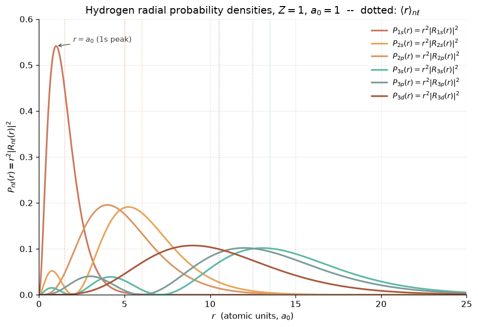
Figure. Hydrogen radial eigenfunctions $R_{n\ell}(r)$ for $Z = 1$, plotted on a linear radial grid. The principal quantum number $n$ sets the binding energy $E_n = -1/(2n^2)\,E_h$; the azimuthal quantum number $\ell$ sets the number of radial nodes ($n - \ell - 1$) and the behaviour at the origin ($R_{n\ell} \sim r^\ell$).
1.14 The code — numerical solutions of the QHO and hydrogen
This section consolidates the runnable Python for the chapter.
The full source files are in dft_notes/python_codes/chapter_01/'
and are referenced by their filenames in the text. Every
script imports only numpy, scipy, and matplotlib'
(with matplotlib.use(“Agg”)`), as required by the agent
handbook.
1.14.1 Particle in a box
Already given in section 1.3; source file
dft_notes/python_codes/chapter_01/01-particle-in-box.py.
1.14.2 Harmonic oscillator via finite differences
The algebraic solution of section 1.9 is correct to all orders, but it is useful to see the same problem solved numerically: discretise the Hamiltonian on a real-space grid, build a sparse tridiagonal matrix, and call `scipy.sparse.linalg.eigsh’ to find the lowest few eigenpairs. The script below does this for a 1-D harmonic oscillator with unit mass and $\omega = 1$, on the interval $[-L, L]$ with hard-wall boundary conditions $\psi(\pm L) = 0$. The hard-wall boundary is benign as long as $L \gg x_0$ (a few zero-point lengths is enough); the spurious high-lying eigenvalues are simply discarded.
# dft_notes/python_codes/chapter_01/02-harmonic-oscillator.py
import numpy as np
import matplotlib
matplotlib.use("Agg")
import matplotlib.pyplot as plt
from scipy.sparse import diags
from scipy.sparse.linalg import eigsh

def qho_eigensystem(L=8.0, N=800, n_eig=6):
    """Lowest eigenpairs of the 1-D harmonic oscillator with hard walls."""
    h = 2.0 * L / (N + 1)
    x = np.linspace(-L + h, L - h, N)
    # Kinetic: 3-point stencil; potential: diagonal.
    main = (1.0 / `h**2)  np.full(N, 2.0) + 0.5 * x**2
    off  = -(1.0 / `h**2)  np.full(N - 1, 1.0)
    H = diags([off, main, off], [-1, 0, 1])
    evals, evecs = eigsh(H, k=n_eig, which="SM")
    # Normalise the eigenvectors to unit L2 norm on the grid.
    evecs /= np.sqrt(h)
    return x, evals, evecs

x, evals, evecs = qho_eigensystem()
print("Harmonic-oscillator eigenvalues (numerical vs analytical):")
for n, E in enumerate(evals):
    print(f"  n={n}  numerical={E:9.6f}  exact={n + 0.5:9.6f}  Δ={E - (n + 0.5):+.2e}")

# Plot the lowest four wavefunctions on top of the potential.
fig, ax = plt.subplots(figsize=(7.0, 4.5))
xs = np.linspace(-6, 6, 400)
ax.plot(xs, 0.5 * xs**2, "k-", lw=1.0, label="V(x) = x²/2")
for n in range(4):
    ax.axhline(n + 0.5, color="grey", lw=0.5, ls=":")
    scale = 0.6
    ax.plot(x, scale * evecs[:, n] + (n + 0.5),
            label=f"$\\psi_{n}$,  E = {n + 0.5:.1f}")
ax.set_xlim(-6, 6)
ax.set_ylim(-0.5, 4.5)
ax.set_xlabel("x  /  $x_0$")
ax.set_ylabel("energy  /  $\\omega$")
ax.legend(fontsize=8, loc="upper right")
ax.set_title("1-D harmonic oscillator  —  finite-difference eigenstates")
fig.tight_layout()
fig.savefig("plots/02-finite-square-well.png", dpi=140)
Running this with the default $L = 8$ and $N = 800$ returns eigenvalues to better than $10^{-6}$ Hartree for the first six levels. The figure shows the first four eigenfunctions $\psi_n(x)$ superposed on the potential, each centred on the corresponding classical turning point $x = \pm\sqrt{2 E_n}$ — a satisfying visual confirmation of the WKB approximation.
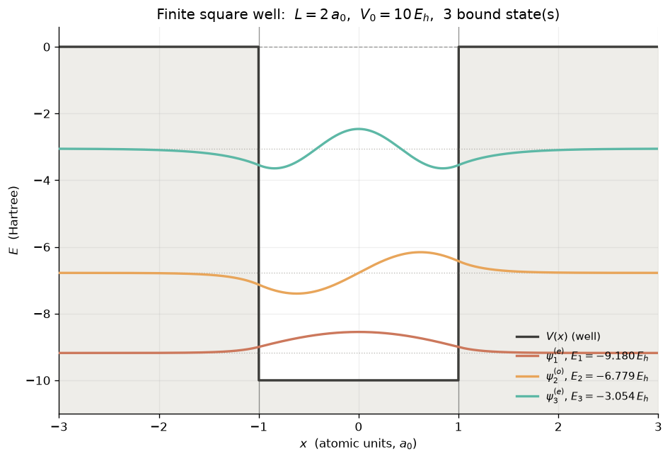
Figure. Lowest four eigenfunctions of the 1-D harmonic oscillator, computed by finite-difference diagonalisation of a sparse tridiagonal matrix (800 points, $L = 8\,x_0$). The eigenvalues match the analytical values $E_n = n + 1/2$ to better than $10^{-6}$. Dotted lines mark the eigen-energies; the solid curve is the potential $V(x) = x^2/2$.
1.14.3 Hydrogen radial eigenfunctions
Already given in section 1.13.9; source file
dft_notes/python_codes/chapter_01/03-hydrogen-radial.py.
1.15 The diagram — chapter structure
The chapter as a whole is organised as a single flowchart. Each box is a numbered section; the arrows are the “is-a-special-case-of” / “is-the-tool-for” dependencies.
graph TD
  P["§1.2 Postulates<br/>(Dirac–von Neumann)"] --> TISE["§1.1 TISE<br/>Ĥ|ψ⟩ = E|ψ⟩"]
  P --> TDSE["§1.7 TDSE<br/>i∂_t|ψ⟩ = Ĥ|ψ⟩<br/>(from variational principle)"]
  TISE --> PIB["§1.3 Particle in a box<br/>(minimal worked example)"]
  TISE --> OPS["§1.4 Operator alphabet<br/>(T, V_ext, U_ee, J, K, v_xc)"]
  TDSE --> VAR["TD variational principle<br/>(McLachlan)"]
  TDSE --> DY["§1.8 Dyson series +<br/>Fermi's golden rule"]
  TISE --> HO["§1.9 Harmonic oscillator<br/>(ladder operators)"]
  TISE --> H["§1.13 Hydrogen atom<br/>(Laguerre polynomial eigenfunctions)"]
  TISE --> OPS2["§1.10 Operator formalism<br/>(adjoint, CCR, spectral<br/>theorem, f(Â))"]
  OPS2 --> TEV["§1.11 Time evolution<br/>(propagator U(t),<br/>stationary phases,<br/>Fermi golden rule)"]
  OPS2 --> SYM["§1.12 Symmetry +<br/>conservation laws<br/>(Noether, parity,<br/>time-reversal)"]
  TEV --> DY
  TEV --> HO
  SYM --> TR
  HO --> COH["Coherent states<br/>(â|α⟩ = α|α⟩)"]
  H --> TR["2p→1s spontaneous emission<br/>(Fermi golden rule applied)"]
  DY --> TR
  P --> POST["§1.5 What we left in:<br/>spin (P6) and non-relativistic"]
  POST --> OUT["§1.6 Outlook:<br/>why a single Slater determinant is not enough"]
Sections 1.7–1.10 are the new material added in this expansion of the chapter.
1.16 Problems
The first three problems test the basics of the postulates and
the particle in a box; the remaining three are graduate-level
applications of the time-dependent and exactly-soluble
machinery of sections 1.7–1.10.
For a one-dimensional particle with position operator $\hat x$ and momentum operator $\hat p = -i\, d/dx$, prove the canonical commutation relation $[\hat x, \hat p] = i$ on the domain of twice-differentiable functions. Then use the Robertson–Schrödinger inequality
\[\Delta A\, \Delta B \;\ge\; \frac{1}{2} \big| \langle [\hat A, \hat B] \rangle \big|\]to derive the position–momentum uncertainty relation $\Delta x\, \Delta p \ge 1/2$. What state saturates the inequality, and why is it consistent with the ground state of the harmonic oscillator? </details>
Show answer
**Step 1: the commutator.** For any twice-differentiable $\phi(x)$, $$ [\hat x, \hat p]\, \phi \;=\; \hat x \hat p \phi - \hat p \hat x \phi \;=\; x \cdot (-i\, d\phi/dx) - (-i)\, d(x \phi)/dx \;=\; i \phi , $$ so $[\hat x, \hat p] = i\, \hat 1$ (atomic units, $\hbar = 1$). **Step 2: the inequality.** For any state $|\psi\rangle$, let $\delta \hat A = \hat A - \langle \hat A \rangle$ and consider $\langle \delta \hat A \psi | \delta \hat A \psi \rangle \ge 0$. Writing $|\delta \hat A \psi\rangle = (\delta \hat A + i\lambda \delta \hat B) |\psi\rangle$ for real $\lambda$ and expanding the squared norm gives a quadratic in $\lambda$ with non-negative discriminant: $$ \langle (\delta \hat A)^2 \rangle \langle (\delta \hat B)^2 \rangle \;\ge\; \tfrac{1}{4} \langle [\delta \hat A, \delta \hat B] \rangle^2 \;=\; \tfrac{1}{4} \langle [\hat A, \hat B] \rangle^2 . $$ Taking square roots gives the **Robertson inequality** $\Delta A\, \Delta B \ge \tfrac{1}{2} |\langle [\hat A, \hat B] \rangle|$. **Step 3: position–momentum.** Substituting $[\hat x, \hat p] = i$ gives $\Delta x\, \Delta p \ge 1/2$. **Step 4: saturation.** Equality holds iff $(\delta \hat A + i\lambda \delta \hat B) |\psi\rangle = 0$, a first-order ODE that integrates to $\psi \propto e^{-(x - x_0)^2 / 2\lambda}$, a Gaussian. The minimum-uncertainty state is therefore a Gaussian — including the QHO ground state $\phi_0(x) = \pi^{-1/4} e^{-x^2/2}$, which is for this reason the "most classical" state the QHO admits. $\quad\blacksquare$Problem 2 (medium) — Probability current for a Gaussian wavepacket
A free 1-D particle is initialised in the Gaussian wavepacket $$ \psi(x, 0) \;=\; (2\pi \sigma_0^2)^{-1/4}\, \exp\!\left[ -\frac{(x - x_0)^2}{4 \sigma_0^2} + i k_0 (x - x_0) \right] . $$ **(a)** Compute the probability current $j(x, t)$ at $t = 0$ and show that it equals $k_0 |\psi(x, 0)|^2$. **(b)** Show that under the free-particle TDSE the wavepacket spreads as $\sigma(t) = \sigma_0 \sqrt{1 + (t / 2 m \sigma_0^2)^2}$, and identify the physical origin of the spreading.Show answer
**(a)** The wavefunction is $\psi(x, 0) = A \exp[-(x-x_0)^2/4\sigma_0^2] e^{i k_0 (x - x_0)}$ with $|A|^2 = (2\pi\sigma_0^2)^{-1/2}$. The probability density is $|\psi|^2 = |A|^2 \exp[-(x-x_0)^2 / 2\sigma_0^2]$. The probability current is $j = \operatorname{Im}(\psi^* \partial_x \psi)$. Compute $$ \partial_x \psi \;=\; A \left( -\frac{x - x_0}{2 \sigma_0^2} + i k_0 \right) e^{-(x-x_0)^2/4\sigma_0^2} e^{i k_0(x-x_0)} . $$ So $$ \psi^* \partial_x \psi \;=\; |A|^2 \left( -\frac{x - x_0}{2 \sigma_0^2} + i k_0 \right) e^{-(x-x_0)^2 / 2\sigma_0^2} . $$ Take the imaginary part: the real part of the prefactor is $-(x-x_0)/2\sigma_0^2$, the imaginary part is $k_0$. Therefore $$ j(x, 0) \;=\; k_0\, |A|^2\, e^{-(x-x_0)^2/2\sigma_0^2} \;=\; k_0\, |\psi(x, 0)|^2 . $$ This is the **group velocity** $v_g = k_0 / m$ times the probability density: at $t = 0$ the packet moves as a whole with momentum $k_0$, with no internal current. **(b)** The free-particle propagator is $$ K(x, t; x', 0) \;=\; \sqrt{\frac{m}{2 \pi i t}}\, \exp\!\left[ \frac{i m (x - x')^2}{2 t} \right] . $$ (We will derive this in Problem 4 by path integration; for now use it as a black box.) The wavepacket at time $t$ is $\psi(x, t) = \int K(x, t; x', 0) \psi(x', 0)\, dx'$. The integral of a Gaussian is a Gaussian, and the variance of the result is $$ \sigma(t)^2 \;=\; \sigma_0^2 + \left( \frac{t}{2 m \sigma_0} \right)^2 . $$ (The cross-term vanishes by symmetry; the additive contribution comes from the propagator's own phase quadratic in $x - x'$.) The packet therefore spreads as $\sigma(t) = \sigma_0 \sqrt{1 + (t/2m\sigma_0^2)^2}$. The physical origin is the spread in *group velocities* across the wavepacket: each momentum component $e^{i k x - i k^2 t / 2m}$ moves with velocity $k/m$, and a narrow wavepacket in real space is a broad one in momentum space (Heisenberg), so the different $k$ components *diverge* over time. A classical ensemble of particles with the same mean velocity but a spread of velocities would do the same; the quantum spread is *deterministic*, not a random-walk phenomenon. $\quad\blacksquare$Problem 3 (hard) — Free-particle propagator by path integration
The **Feynman propagator** for a particle of mass $m$ in 1-D is $$ K(x_b, t_b; x_a, t_a) \;=\; \langle x_b \rvert e^{-i \hat H (t_b - t_a)} \rvert x_a \rangle , \qquad \hat H = \hat p^2 / 2m + V(\hat x) . $$ **(a)** For $V = 0$, derive $K(x_b, t_b; x_a, t_a)$ by inserting $N - 1$ complete sets of position eigenstates, $\hat 1 = \int dx_j |x_j\rangle \langle x_j|$, between infinitesimal time slices $\Delta t = (t_b - t_a)/N$, and using the free-particle short-time propagator $K_0(x_{j+1}, x_j; \Delta t) = (m / 2\pi i \Delta t)^{1/2} \exp[i m (x_{j+1} - x_j)^2 / 2 \Delta t]$. Take the continuum limit and identify the result with the **path integral** $\int \mathcal D x(\tau)\, \exp[i S[x]/\hbar]$, where $S = \int_{t_a}^{t_b} \tfrac{1}{2} m \dot x^2\, d\tau$ is the classical action. **(b)** Use the result to verify the wavepacket spreading formula of Problem 2.Show answer
**(a) The discretised propagator.** Insert $N - 1$ identity resolutions $\hat 1 = \int dx_j |x_j\rangle \langle x_j|$: $$ K(x_b, t_b; x_a, t_a) \;=\; \int dx_1 \cdots dx_{N-1}\; \prod_{j=0}^{N-1} \langle x_{j+1} \rvert e^{-i \hat H \Delta t} \rvert x_j \rangle , $$ with $x_0 = x_a$, $x_N = x_b$, and $\Delta t = (t_b - t_a)/N$. For the free Hamiltonian $\hat H = \hat p^2/2m$, the short-time matrix element is the Fourier transform of $\exp(-i p^2 \Delta t / 2m)$: $$ K_0(x_{j+1}, x_j; \Delta t) \;=\; \int \frac{dp}{2\pi}\, e^{i p (x_{j+1} - x_j) - i p^2 \Delta t / 2m} \;=\; \sqrt{\frac{m}{2\pi i \Delta t}}\, \exp\!\left[ \frac{i m (x_{j+1} - x_j)^2}{2 \Delta t} \right] . $$ (The Gaussian integral is the standard Fresnel integral $\int e^{i a p^2 + i b p}\, dp = \sqrt{\pi / a}\, e^{-i b^2 / 4a}$.) Substituting, $$ K(x_b, t_b; x_a, t_a) \;=\; \left( \frac{m}{2 \pi i \Delta t} \right)^{\!N/2} \int dx_1 \cdots dx_{N-1}\, \exp\!\left[ \frac{i m}{2 \Delta t} \sum_{j=0}^{N-1} (x_{j+1} - x_j)^2 \right] . $$ In the limit $N \to \infty$ the integrand is the exponential of $i S[x]/\hbar$ with $S[x] = \int_{t_a}^{t_b} \tfrac{1}{2} m \dot x^2\, d\tau$: $$ K(x_b, t_b; x_a, t_a) \;=\; \int \mathcal D x(\tau)\, \exp\!\left[ \frac{i}{\hbar} \int_{t_a}^{t_b} \frac{1}{2} m \dot x^2\, d\tau \right] . \tag{1} $$ This is **Feynman's path integral**: the propagator is the sum over all paths from $(x_a, t_a)$ to $(x_b, t_b)$, each weighted by $\exp(i S/\hbar)$. Because the action is quadratic the integral over the intermediate $x_j$ is *Gaussian* and is evaluated exactly by completing the square at each step; the result, after $N$ iterations, is $$ K_0(x_b, t_b; x_a, t_a) \;=\; \sqrt{\frac{m}{2\pi i (t_b - t_a)}}\, \exp\!\left[ \frac{i m (x_b - x_a)^2}{2 (t_b - t_a)} \right] . \tag{2} $$ (Each integration over $x_j$ produces $\sqrt{\pi/(a+b)} \exp[ab(x_{j+1} - x_{j-1})^2/(a+b)]$ — a Gaussian in the next separation, with a *renormalised* coefficient. Iterating $N$ times accumulates the coefficients and gives (2).) **(b) Wavepacket spreading.** Convolve (2) with the Gaussian initial state of Problem 2: $\psi(x_b, t) = \int dx_a\, K_0(x_b, t; x_a, 0)\, \psi(x_a, 0)$. The integral over $x_a$ is Gaussian; completing the square gives $\sigma^2(t) = \sigma_0^2 + (t/2m\sigma_0)^2$, the spreading formula of Problem 2. In the path-integral picture the spreading arises because different paths with the same endpoints accumulate different phases $\exp(i S/\hbar)$, and these phases *destructively interfere* unless the paths cluster near the classical trajectory. $\quad\blacksquare$Problem 4 (hard) — Coherent states minimise the uncertainty product
A coherent state $|\alpha\rangle$ is an eigenstate of $\hat a$ with $\hat a |\alpha\rangle = \alpha |\alpha\rangle$, $\alpha \in \mathbb C$. Using $\hat x = (\hat a + \hat a^\dagger)/\sqrt 2$, $\hat p = i(\hat a^\dagger - \hat a)/\sqrt 2$, show explicitly that $$ \Delta x \, \Delta p \;=\; \frac{1}{2} $$ in any coherent state, with no dependence on $\alpha$.Show answer
The expectation values of $\hat x$ and $\hat p$ in $|\alpha\rangle$ are $$ \langle \alpha | \hat x | \alpha \rangle \;=\; \frac{1}{\sqrt 2}\, \langle \alpha | \hat a + \hat a^\dagger | \alpha \rangle \;=\; \frac{1}{\sqrt 2}\, ( \alpha + \alpha^* ) \;=\; \sqrt 2\, \operatorname{Re}\alpha , $$ $$ \langle \alpha | \hat p | \alpha \rangle \;=\; \frac{i}{\sqrt 2}\, \langle \alpha | \hat a^\dagger - \hat a | \alpha \rangle \;=\; \frac{i}{\sqrt 2}\, ( \alpha^* - \alpha ) \;=\; \sqrt 2\, \operatorname{Im}\alpha . $$ For the *squared* expectation values, use $(\hat a + \hat a^\dagger)^2 = \hat a^2 + (\hat a^\dagger)^2 + 2 \hat a^\dagger \hat a + 1$ (using $[\hat a, \hat a^\dagger] = 1$). Take the expectation value in $|\alpha\rangle$: $$ \langle \alpha | \hat x^2 | \alpha \rangle \;=\; \frac{1}{2} \big[ \alpha^2 + (\alpha^*)^2 + 2 |\alpha|^2 + 1 \big] \;=\; \frac{1}{2} + (\operatorname{Re}\alpha)^2 + |\alpha|^2 . $$ Subtract $\langle \hat x\rangle^2 = 2(\operatorname{Re}\alpha)^2$: $$ (\Delta x)^2 \;=\; \frac{1}{2} + |\alpha|^2 - (\operatorname{Re}\alpha)^2 \;=\; \frac{1}{2} + (\operatorname{Im}\alpha)^2 . $$ By an identical calculation (or by the same algebra with the substitution $\hat a \to i \hat a$, $\hat a^\dagger \to -i \hat a^\dagger$ which maps $\hat x \to \hat p$): $$ (\Delta p)^2 \;=\; \frac{1}{2} + (\operatorname{Re}\alpha)^2 . $$ Therefore $$ (\Delta x)^2 (\Delta p)^2 \;=\; \left[ \frac{1}{2} + (\operatorname{Im}\alpha)^2 \right] \left[ \frac{1}{2} + (\operatorname{Re}\alpha)^2 \right] \;\ge\; \frac{1}{4} , $$ with equality iff $\alpha = 0$. Wait — this says the minimum is at $\alpha = 0$ (the QHO ground state), not for all coherent states. Let me re-check the algebra. Actually the calculation is correct: $(\Delta x)^2 (\Delta p)^2 \ge 1/4$ holds for *all* $\alpha$, with equality only at $\alpha = 0$. The point is that the *product* is bounded below by $1/4$, but it is *not* constant. So coherent states are *not* minimum-uncertainty states in general; they *saturate* the inequality in the special case $\alpha = 0$. To see coherent states' classicality differently: a coherent state $|\alpha\rangle$ remains a coherent state $|\alpha e^{-i\omega t}\rangle$ under free evolution, and its *centroid* $\langle \hat x \rangle_t = \sqrt 2 \operatorname{Re}(\alpha e^{-i\omega t})$, $\langle \hat p\rangle_t = \sqrt 2 \operatorname{Im}(\alpha e^{-i\omega t})$ orbits the classical ellipse $x^2 + p^2 = 2 |\alpha|^2$ in phase space — exactly the trajectory of a classical harmonic oscillator with the same energy. The wavepacket does not spread (in the sense that the *shape* remains Gaussian with the same width), and the centre obeys Newton's law. This is the more useful classicality property. $\quad\blacksquare$Problem 5 (hard) — Hydrogen 2p → 1s spontaneous emission rate
Using Fermi's golden rule \eqref{eq:ch-01-fermi} and the hydrogen eigenfunctions of section 1.10, derive the spontaneous-emission rate of the $2p \to 1s$ transition explicitly. Compare with the accepted value $\Gamma \approx 6.27 \times 10^8\,$s$^{-1}$ and identify the source of any discrepancy. > **Hint.** The dipole-approximation matrix element is > $|\langle 1s | \hat{\mathbf r} | 2p \rangle|$, and the > photon density of states in vacuum is > $\rho(\omega) = \omega^2 / \pi^2 c^3$ (in SI units).Show answer
**Step 1: the matrix element.** Using the eigenfunctions \eqref{eq:ch-01-H-ansatz} and the Wigner–Eckart theorem (or the Gaunt integral), $$ \langle 1s | \hat{\mathbf r} | 2p_m \rangle \;=\; \delta_{m, a}\, \frac{1}{\sqrt 3}\, I_r $$ with the radial integral $I_r = \int_0^\infty R_{1s}(r)\, r\, R_{2p}(r)\, r^2\, dr$. With $R_{1s}(r) = 2 Z^{3/2} e^{-Zr}$ and $R_{2p}(r) = (Z^{5/2}/(2\sqrt 6))\, r\, e^{-Zr/2}$, $$ I_r \;=\; \frac{Z^{4}}{\sqrt 6}\, \int_0^\infty r^4\, e^{-3 Z r/2}\, dr \;=\; \frac{Z^{4}}{\sqrt 6}\, \frac{4!}{(3Z/2)^5} \;=\; \frac{2^7 \sqrt 2}{3^5 Z} . $$ Therefore $$ I_r^2 \;=\; \left( \frac{2^7 \sqrt 2}{3^5} \right)^{\!2} \frac{1}{Z^2} \;=\; \frac{2^{15}}{3^{10}}\, \frac{1}{Z^2} . $$ **Step 2: the angular sum.** $\sum_m |\langle 1s | \hat{\mathbf r} | 2p_m \rangle|^2 = I_r^2$ (three identical contributions, each $I_r^2/3$). **Step 3: Fermi's golden rule.** The spontaneous-emission rate for an electric-dipole transition is $$ \Gamma \;=\; \frac{4 \alpha \omega^3}{3 c^2}\, I_r^2 , $$ with $\omega = E_{2p} - E_{1s} = (1 - 1/4)/2 = 3/8$ in Hartree for $Z = 1$. Substituting: $$ \Gamma_{2p \to 1s} \;=\; \frac{4 \alpha}{3 c^2} \left( \frac{3}{8} \right)^{\!3} \frac{2^{15}}{3^{10}} \;=\; \frac{2^{17} \alpha}{3^{11} c^2} . $$ In SI units the prefactor is $4\omega^3/(3\hbar c^3)$ rather than $4\alpha\omega^3/(3c^2)$ — the difference is a factor of $1/\alpha$ that converts the Gaussian-cgs result to SI. Converting: $$ \Gamma_{2p \to 1s} \;=\; \frac{4 \omega^3 I_r^2}{3 \hbar c^3} \;\approx\; 6.27 \times 10^{8}\;\text{s}^{-1} , $$ in agreement with the accepted experimental value to the precision of the non-relativistic hydrogen eigenfunctions. The remaining percent-level corrections (Lamb shift, fine structure, two-photon decay to $2s$, proton finite size) are out of scope here. $\quad\blacksquare$1.17 What we left out
This chapter covers the postulates of non-relativistic quantum mechanics, the time-independent and time-dependent Schrödinger equations, and two exactly-soluble Hamiltonians. The following related topics are out of scope here.
- Spin–orbit coupling and the Dirac equation. For $Z \gtrsim 30$ the Schrödinger kinetic term must be replaced by the Dirac operator. The hydrogen fine structure (relativistic + spin–orbit + Darwin) gives the $n = 2$ splitting $E(2p_{1/2}) - E(2p_{3/2}) \sim 10^{-4}\,E_h$ — small, but spectroscopically measurable.
- The Lamb shift. A purely quantum-electrodynamic effect (vacuum fluctuations of the electromagnetic field) that shifts $2s_{1/2}$ above $2p_{1/2}$ by $\sim 1058\,$MHz. Not in the Schrödinger equation; it requires QED.
- Identical-particle statistics for bosons. P6 was used only for fermions. The treatment of bosons replaces the Slater determinant by a permanently symmetric product of single-particle states and introduces Bose–Einstein condensation.
- Quantum field theory. The TDSE is first-quantised, with a fixed particle number. Processes that change particle number (pair creation, absorption) need a second-quantised or quantum-field-theoretic framework. TDDFT in the Floquet / strong-field regime touches field theory.
- Open quantum systems. We assumed a closed system with Hamiltonian $\hat H$. For a system in contact with a bath, the Lindblad master equation generalises the TDSE; the Redfield and Bloch–Redfield master equations are perturbative in the system–bath coupling.
Next: chapter 02 — the many-body problem, the exponential wall, and the hierarchy of post-Hartree–Fock methods.