Chapter 10 — Phonons & vibrations

The nuclei in a solid are not static. They oscillate around their equilibrium positions with small amplitudes, and these oscillations are quantised: the energy comes in lumps, $\hbar \omega_s(\mathbf q)$, called phonons. This chapter is the construction of the dispersion $\omega_s(\mathbf q)$ from first principles — the dynamical matrix $D(\mathbf q)$ that is to vibrations what the Hamiltonian is to electrons.

By the end of chapter 09 we had a procedure for finding the equilibrium geometry of a molecule or solid: minimise the Kohn–Sham total energy $E[{\mathbf R_I}]$ with respect to the nuclear positions ${\mathbf R_I}$. The minimum of $E$ defines the ground-state geometry $\mathbf R_I^{(0)}$. Around this minimum the energy has a quadratic form, so a small displacement of one nucleus produces a restoring force on every other nucleus. The matrix of these second derivatives, $\partial^2 E / \partial R_{I\alpha} \partial R_{J\beta}$ (where $\alpha, \beta \in {x, y, z}$), is called the force-constant matrix $\Phi_{I\alpha, J\beta}$. It is the spring constant of the solid.

This chapter turns $\Phi$ into a dynamical matrix $D(\mathbf q)$ by a Fourier transform, and diagonalises $D(\mathbf q)$ at every phonon wavevector $\mathbf q$ in the Brillouin zone to obtain the phonon dispersion $\omega_s(\mathbf q)$ — the analogue of the electronic band structure $\varepsilon_n(\mathbf k)$ of chapter 07. The plan is: (1) state the claim; (2) introduce the frozen-phonon method (§10.2), in which the force-constant matrix is built from a finite number of supercell force calculations; (3) explain the linear-response method (DFPT, §10.3) that gives $\Phi$ for any $\mathbf q$ from a single unit cell; (4) give the acoustic sum rule (§10.4) and the LO-TO splitting (§10.5) that pin down $\omega_s(\mathbf q)$ at the two limits $\mathbf q \to 0$ and $\mathbf q = 0$ for ionic crystals; (5) connect the dispersion to the *phonon density of states and the thermodynamic* functions (§10.6); (6) sketch the anharmonic corrections that go beyond the harmonic approximation (§10.7); and (7) treat the electron-phonon coupling (§10.8) that ties phonons back to electrons and opens the door to superconductivity.

Reading note. This chapter assumes chapter 07 (Bloch theorem, Brillouin zone, k-point sampling) and chapter 09 (Hellmann–Feynman forces, geometry optimisation). It uses concepts from chapter 04 (Kohn–Sham DFT) and chapter 08 (pseudopotentials).

10.1 The claim

Phonons are the normal modes of small nuclear displacements around the equilibrium geometry of a solid. Their frequencies $\omega_s(\mathbf q)$ at a given phonon wavevector $\mathbf q$ and branch index $s$ are the eigenvalues of the dynamical matrix

\[\begin{equation} \label{eq:ch-10-dyn-def} D_{I\alpha, J\beta}(\mathbf q) \;=\; \frac{1}{\sqrt{M_I M_J}}\, \tilde\Phi_{I\alpha, J\beta}(\mathbf q) , \end{equation}\]

where $\tilde\Phi$ is the Fourier transform of the real-space force-constant matrix

\[\begin{equation} \label{eq:ch-10-fc-def} \Phi_{I\alpha, J\beta}(\mathbf R) \;\equiv\; \frac{\partial^2 E}{\partial R_{I\alpha}^{(0)} \, \partial R_{J\beta}^{(\mathbf R)}} , \end{equation}\]

$M_I$ is the mass of nucleus $I$, and $E$ is the Kohn–Sham total energy in the Born–Oppenheimer approximation.

The rest of this section unpacks the claim. The proof that $\omega_s(\mathbf q)$ comes from the eigenvalues of \eqref{eq:ch-10-dyn-def} is the content of §10.1.2; the link between $\Phi$ and the Kohn–Sham energy is the force theorem of chapter 09 §9.4; the matrix $\tilde\Phi$ and its relation to $\Phi$ is the discrete Fourier transform derived in §10.1.3. ### 10.1.1 Why a Fourier transform?

The solid is infinite. We want a wavevector $\mathbf q$ to label the modes by crystal momentum (the phonon analogue of the electronic $\mathbf k$ of chapter 07). For a 1-D chain of $N$ atoms with mass $M$ and lattice constant $a$, Bloch’s theorem says a normal mode with wavevector $q$ has the form

i.e. the displacement of atom $n$ is a plane wave in $n$ modulated by an amplitude $U_{s\alpha}(q)$ that is the same in every cell. This ansatz is exact if $\Phi$ is translationally invariant — i.e. if the force constant between atom $n$ and atom $m$ depends only on $m - n$, which is true for a perfect crystal.

The ansatz is what makes the dynamical matrix finite (size $3 N_\text{atom}$ per unit cell, where $N_\text{atom}$ is the number of atoms in the primitive cell) at every $\mathbf q$. Without it, we would have a $3N$-by-$3N$ matrix for a solid of $N$ atoms (an integer that diverges in the thermodynamic limit). The Fourier transform from real-space force constants $\Phi_{I\alpha, J\beta}(\mathbf R)$ to dynamical matrix elements $D_{I\alpha, J\beta}(\mathbf q)$ is the operation that takes advantage of the translational symmetry to reduce an infinite matrix to a $3 N_\text{atom}$-by-$3 N_\text{atom}$ matrix indexed by atom within one cell.

10.1.2 The equation of motion

Expand the Born–Oppenheimer energy of chapter 01 to second order in the nuclear displacements $u_{I\alpha} = R_{I\alpha} - R_{I\alpha}^{(0)}$ around the equilibrium geometry:

(The first-order terms vanish at the equilibrium geometry; the definition of $\Phi$ is the second derivative, equation \eqref{eq:ch-10-fc-def}, which is a Hessian of the energy landscape.)

The classical equation of motion for nucleus $I$ in direction $\alpha$ is Newton’s law,

Substituting the Bloch ansatz $u_{I\alpha}(t) = U_{s\alpha}(q)\, e^{i(q R_I - \omega_s(q) t)}$ (where $R_I$ here denotes the position of atom $I$ within the supercell) and using $\ddot u_{I\alpha} = -\omega_s^2 u_{I\alpha}$, we get

Define the dynamical matrix

with the Fourier transform

Equation \eqref{eq:ch-10-eom-bloch} is then the eigenvalue problem

The eigenvalues of $D(\mathbf q)$ are $\omega_s^2(\mathbf q)$, with $s = 1, 2, \ldots, 3 N_\text{atom}$ (three branches per atom in the primitive cell). The corresponding eigenvectors $U_s(q)$ are the polarisation vectors of the mode.

Note. We wrote the equation of motion with $\Phi_{I\alpha, J\beta}(\mathbf 0)$ — the on-site force constant. The Fourier transform \eqref{eq:ch-10-fc-fourier} will re-introduce the off-cell matrix elements in the standard way. The argument generalises straightforwardly to multiple atoms per cell; the only change is that the index $J$ now runs over all atoms in the crystal (i.e. over all $N_\text{atom}$ atoms in every cell), and the matrix $D(\mathbf q)$ is $3N_\text{atom} \times 3N_\text{atom}$ in size.

10.1.3 The Fourier transform in practice

For a perfect crystal under Born–von Karman boundary conditions (chapter 07), the force-constant matrix is invariant under simultaneous translation of the unit-cell labels:

The discrete Fourier transform from the relative-cell index to the phonon wavevector $\mathbf q$ is then

(Here $\Phi_{I\alpha, J\beta}(\mathbf R)$ is the force constant between atom $I$ in the reference cell and atom $J$ in the cell $\mathbf R$ away.) The phonon wavevectors $\mathbf q$ live on the same Monkhorst–Pack mesh as the electronic $\mathbf k$ of chapter 07 §7.6 — i.e. on a uniform mesh in the first Brillouin zone of the primitive lattice, with $N_\mathbf q$ points per BZ where $N_\mathbf q = N_1 N_2 N_3$ in the Born–von Karman supercell.

Tip. The convention for the sign in \eqref{eq:ch-10-dft} varies by author. We use $e^{-i\mathbf q\cdot\mathbf R}$ for the cell-phase, so that the Bloch ansatz $u_{I\alpha}(t) = U_{s\alpha}(q)\, e^{i(\mathbf q\cdot\mathbf R_I - \omega t)}$ is positive-frequency (i.e. travels in the direction of $\mathbf q$). Some authors use the opposite sign; both are correct as long as they are used consistently in \eqref{eq:ch-10-dyn-eig} and \eqref{eq:ch-10-dft}.

10.2 The frozen-phonon method

The frozen-phonon method builds the force-constant matrix by explicitly displacing atoms and computing the forces that result. It is conceptually the simplest route from a DFT code to a phonon dispersion, and it is the one that ties most directly to the forces machinery of chapter 09.

10.2.1 The supercell trick

Phonons with wavevector $\mathbf q$ in the primitive BZ are commensurate with a supercell of size $L \mathbf a$ along the direction of $\mathbf q$, where $L$ is the smallest integer such that $L \mathbf a \cdot \mathbf q = 2\pi m$ for some integer $m$ (in 1-D: $L a q = 2\pi m$, so $L = m \cdot 2\pi / (q a)$). For a general $\mathbf q$, $L$ is infinite and the supercell is the infinite crystal. The frozen-phonon approach handles this by approximating a general $\mathbf q$ by a commensurate one in a finite supercell.

Concretely: pick a supercell of $L_1 \times L_2 \times L_3$ primitive cells. Apply the Bloch ansatz $u_{I\alpha}(\mathbf R) = U_\alpha(\mathbf R) e^{i\mathbf q\cdot \mathbf R}$ exactly — i.e. the same amplitude $U_\alpha$ is applied to every copy of atom $I$ in the cell $\mathbf R$ (modulo the phase factor $e^{i\mathbf q\cdot\mathbf R}$). This is a perfectly periodic distortion of the supercell, so a single SCF calculation in the supercell gives the force on every atom in the supercell. The forces are then interpreted as the forces at the corresponding $\mathbf q$ in the primitive cell.

Note. The commensurate approximation works for any $\mathbf q$ that is a rational multiple of a reciprocal-lattice vector. The discrete set of $\mathbf q$ values you can reach is determined by the supercell size: an $L_1 \times L_2 \times L_3$ supercell gives a $\mathbf q$-mesh of $L_1 \times L_2 \times L_3$ points in the BZ (analogous to the BvK mesh for electronic $\mathbf k$ in chapter 07). To compute the dispersion at a fine $\mathbf q$-mesh you need a correspondingly large supercell — which is the practical bottleneck of the frozen-phonon method.

10.2.2 From forces to the force-constant matrix

A single force calculation tells you the force on each atom induced by a particular displacement pattern, not the second derivative directly. To extract the second derivative, you need two displacement patterns and a finite-difference fit, or you need to invert the relationship

by computing $F$ for enough linearly independent displacement patterns $u$ that the linear system for $\Phi$ becomes determined or over-determined.

The simplest recipe is the finite-difference central-difference formula: for each atom $I$ and each Cartesian direction $\alpha$, apply the displacement $u_{J\beta} = \pm \delta\, \delta_{IJ} \delta_{\alpha\beta}$ (i.e. displace atom $I$ by $\pm \delta$ in direction $\alpha$ and only that atom), and compute the resulting forces. The off-diagonal element $\Phi_{I\alpha, J\beta}$ for $J \neq I$ is then

where $F_{I\alpha}(\pm \delta_{J\beta})$ is the force on atom $I$ in direction $\alpha$ after atom $J$ has been displaced by $\pm \delta$ in direction $\beta$. For the diagonal element $\Phi_{I\alpha, I\alpha}$, the displacement is along the same direction as the force, and the same formula applies. The finite-difference step $\delta$ is typically $0.01$–$0.05$ Å.

The total number of force calculations required by the single- atom finite-difference scheme is $2 \times 3 N_\text{atom-in-cell}$ for a primitive cell and $2 \times 3 N_\text{atom-in-supercell}$ for a supercell. By the symmetry of $\Phi$ (it is symmetric in $I\alpha \leftrightarrow J\beta$), this can be halved.

Warning. The single-atom finite-difference scheme misses any force-constant matrix element that connects atoms in different supercell images when only one atom is displaced. To get the inter-cell force constants $\Phi_{I\alpha, J\beta}(\mathbf R)$ for $\mathbf R \neq 0$, you must use a supercell large enough to fit the longest-ranged force constant you want to resolve. For insulators the force constants are usually short-ranged (a few Å), but for metals the long-range Friedel oscillations in the dielectric response make the force constants effectively long-ranged; the supercell must be sized accordingly or periodic-image interactions will pollute the fit.

10.2.3 The Fourier transform back to $D(\mathbf q)$

Once the full force-constant matrix $\Phi_{I\alpha, J\beta}(\mathbf R)$ is in hand, the dynamical matrix is obtained by the discrete Fourier transform \eqref{eq:ch-10-dft}. In a frozen-phonon calculation on a commensurate supercell, the $\mathbf q$ that the supercell supports are exactly the discrete set ${\mathbf q_\text{mesh}}$ corresponding to the supercell, so the Fourier transform is just a sum over the supercell cells:

Diagonalising $D(\mathbf q_\text{mesh})$ for every $\mathbf q_\text{mesh}$ gives the phonon frequencies at those mesh points. The dispersion along a high-symmetry path (e.g. $\Gamma \to X \to M \to \Gamma$ in a cubic BZ) is then obtained by interpolation, or by re-fourier-interpolating $\Phi$ to a finer $\mathbf q$-mesh and diagonalising again. The latter is the Fourier-interpolation method of Gonze, Charlier, Allan, Teter (1994), and is the standard way to get a smooth dispersion curve from a finite-supercell frozen-phonon calculation.

10.2.4 Diagram — the frozen-phonon workflow

The frozen-phonon route from a converged ground-state calculation to a phonon dispersion is a sequence of $O(N_\text{atom})$ displacement-force pairs, followed by a Fourier interpolation. The box below summarises the pipeline; every box is one full self-consistent field (SCF) calculation on a supercell.

%%{init: {'flowchart': {'htmlLabels': true, 'curve': 'basis'}}}%%
graph TD
  R0["Equilibrium geometry<br/>R(0), a(0)<br/>(chapter 09)"] --> SCF0["SCF on primitive cell<br/>yields E(0) and rho(0)"]
  SCF0 --> SUPC["Build supercell<br/>L1 x L2 x L3 primitive cells<br/>(commensurate with q-mesh)"]
  SUPC --> LOOP["For each atom I and<br/>Cartesian direction alpha:<br/>displace by +/- delta"]
  LOOP --> DISP["Apply Bloch ansatz<br/>u(R) = U e^{iq.R}<br/>(commensurate q)"]
  DISP --> SCF1["SCF on supercell<br/>with frozen displacement<br/>(one full KS solve)"]
  SCF1 --> FORCES["Extract forces F_I on every atom<br/>(Hellmann-Feynman,<br/>chapter 09)"]
  FORCES --> FIT["Fit force constants<br/>Phi(R) = (F(+d) - F(-d)) / 2d"]
  FIT --> NEXT{"More I, alpha?"}
  NEXT -->|yes| LOOP
  NEXT -->|no| FFT["Fourier transform<br/>Phi(R) -> D(q)<br/>discrete sum on supercell"]
  FFT --> DIAG["Diagonalise D(q)<br/>at each commensurate q<br/>yields omega_s(q)"]
  DIAG --> OUT["Phonon dispersion<br/>omega_s(q) at supercell q-points"]

  classDef input fill:#eef0e6,stroke:#3a4031,color:#1c1f17;
  classDef scf   fill:#d6dcc8,stroke:#3a4031,color:#1c1f17;
  classDef out   fill:#cc785c,stroke:#1c1f17,color:#ffffff;
  class R0 input
  class SCF0 input
  class SUPC scf
  class LOOP scf
  class DISP scf
  class SCF1 scf
  class FORCES scf
  class FIT scf
  class NEXT scf
  class FFT scf
  class DIAG scf
  class OUT out

The inner loop LOOP’ is the cost driver: it runs $2 \times 3 N_\text{atom-in-supercell}$ independent SCF calculations. By symmetry of $\Phi$ (which is symmetric under $I \leftrightarrow J$, $\alpha \leftrightarrow \beta$) this can be halved. The outer box FFT’ is the cheap step (a single discrete Fourier transform), and DIAG’ is one matrix diagonalisation per $\mathbf q$. The set of $\mathbf q$ values reachable is the commensurate set determined by the supercell — to resolve a finer $\mathbf q$-mesh one must use a larger supercell, which is the bottleneck of the method.

10.3 Density-functional perturbation theory (DFPT)

The frozen-phonon method has a cost that grows with the supercell size — linearly with the number of atoms, but the number of distinct force calculations is $O(N_\text{atom})$ and each force calculation is an entire SCF cycle on a supercell. A phonon dispersion along a high-symmetry path of length 6–10 segments requires $O(10)$ supercell SCF calculations at $O(10)$ supercell sizes — easily $O(100)$ SCF cycles in total. The density-functional perturbation theory (DFPT) approach of Baroni, Giannozzi, Testa (1987) and Gonze (1995) gets the same force-constant matrix from a single unit-cell calculation by solving a linear-response problem for the self-consistent potential at every $\mathbf q$.

10.3.1 The $2n + 1$ theorem

DFPT rests on a deep formal result. Consider a static perturbation parameter $\lambda$ that couples to the system through some one-electron operator $\partial \hat V_\lambda / \partial \lambda$. The $2n + 1$ theorem (or “third-order analyticity” theorem, see Gonze & Vigneron (1989)) states that the $2n+1$-th derivative of the total energy with respect to $\lambda$ can be computed from a knowledge of the wave- function perturbed to only order $n$:

For phonons, $\lambda$ is the amplitude of a nuclear displacement with wavevector $\mathbf q$, and the relevant quantity is the second derivative of the energy ($n = 1$, $2n + 1 = 3$, but we want $\partial^2 E$ — see below). The $2n + 1$ theorem guarantees that the second derivative of the energy is computable from a knowledge of only the first-order change in the wavefunction $\psi^{(1)}$, which in turn is determined by a single linear equation (the Sternheimer equation, §10.3.2) — not by a separate self-consistent calculation at each amplitude.

In practice the $2n + 1$ theorem is invoked differently. The first derivative of the energy (the force) is the Hellmann– Feynman theorem of chapter 09. The second derivative (the force-constant matrix) is $2n + 1$ for $n = 0$ (since $2(0) + 1 = 1$, but we want the 2nd derivative — so the theorem is sometimes stated as: “the energy to order $2n+1$ requires the wavefunction to order $n$”, which for the force-constant matrix ($n = 0$ for the second derivative of the energy) means no wavefunction perturbation at all — but the force-constant matrix itself is second-order in the perturbation amplitude, so we need $\psi^{(1)}$ to compute it). Either way, the practical consequence is the same: a single linear-response calculation gives the second derivative of the energy with respect to every perturbation of the chosen wavevector.

10.3.2 The Sternheimer equation

Let $\hat H^{(0)}$ be the unperturbed Kohn–Sham Hamiltonian, with eigenstates $\psi_n^{(0)}$ and eigenvalues $\varepsilon_n^{(0)}$. Apply a small static perturbation with wavevector $\mathbf q$ and amplitude $\lambda$ (think of a phonon displacement $\mathbf u_{I\alpha} = \lambda\, e^{i\mathbf q\cdot\mathbf R_I} \hat{\mathbf e}_\alpha$). The first-order change in the Hamiltonian is $\hat H^{(1)} = \partial \hat H / \partial \lambda$ at $\lambda = 0$. The first-order change in the wavefunction $\psi_n^{(1)}$ satisfies the Sternheimer equation

where $\varepsilon_n^{(1)} = \langle \psi_n^{(0)} \rvert \hat H^{(1)} \rvert \psi_n^{(0)} \rangle$ is the first-order change in the eigenvalue (the Hellmann–Feynman contribution to the force on the displaced nucleus). The operator on the left is singular (it has a zero eigenvalue corresponding to $\psi_n^{(0)}$ itself); the standard fix is to project out the $\psi_n^{(0)}$ component and solve in the orthogonal complement of the unperturbed eigenstate. This is a linear equation in $\psi_n^{(1)}$, not a self-consistent one — but the Hamiltonian $\hat H^{(0)}$ depends on the density $\rho$, so the self-consistent density response $\rho^{(1)}$ couples all the $\psi_n^{(1)}$ together through the Hartree and exchange–correlation potentials. The self-consistent Sternheimer equation is

with $\hat V_\text{Hxc}^{(1)}[\rho^{(1)}]$ the linear change in the Hartree+XC potential induced by the linear density response $\rho^{(1)} = \sum_n^\text{occ} \psi_n^{(0)*} \psi_n^{(1)} + \text{c.c.}$.

The Sternheimer equation is solved iteratively: start with $\hat V_\text{Hxc}^{(1)} = 0$, solve for $\psi_n^{(1)}$, build $\rho^{(1)}$, rebuild $\hat V_\text{Hxc}^{(1)}[\rho^{(1)}]$, and iterate to self-consistency. The cost is one linear-response cycle per $\mathbf q$ point, comparable to a single SCF iteration in a regular ground-state calculation.

10.3.3 The dynamical matrix from DFPT

Once the self-consistent first-order density response $\rho^{(1)}$ is known, the second derivative of the energy with respect to the phonon amplitude follows from the $2n + 1$ theorem applied at $n = 0$ for the second derivative, or by direct application of the $2n + 1$ formula for the second derivative:

(Here $\partial \hat H_I$ is the derivative of the Hamiltonian with respect to the displacement of atom $I$ in the chosen direction; the result is a Hessian of the energy with respect to the displacement amplitudes, which is the force-constant matrix element $\Phi_{I\alpha, J\beta}$ in the limit $\mathbf q = 0$ or its Fourier transform in general.)

The crucial point is that the only piece of \eqref{eq:ch-10-dyn-dfpt} that depends on the self-consistent response is the second term with $\psi_n^{(1)}$. The first term — the “bare” second derivative of the Hamiltonian, which includes the change in the external potential when the nuclei are displaced — is known analytically (it is the change in the electron-nucleus Coulomb attraction plus the change in the nucleus-nucleus repulsion). So the entire self-consistent machinery is just the Sternheimer equation, and the force constant is a post-processing of $\psi_n^{(1)}$.

Tip. DFPT is implemented in production codes like Quantum ESPRESSO, ABINIT, and CASTEP under the keyword ‘phonon’ / ‘dfpt’ / ‘linear response’. For each $\mathbf q$ the code runs one Sternheimer SCF cycle (linear in the occupied states) and outputs the dynamical matrix. The cost of a full phonon dispersion is then $N_\mathbf q$ linear calculations, not $N_\mathbf q$ non-linear ones — a savings of a factor of 5–10 per $\mathbf q$ over a frozen-phonon approach.

10.3.4 Why DFPT scales better

The frozen-phonon method requires a separate supercell calculation for each $\mathbf q$, and the supercell grows without bound as one moves to fine $\mathbf q$ meshes. The DFPT method always works in the primitive cell (or the unit cell of the perturbation), and the cost grows only with the size of the basis needed to represent the self-consistent response. For a plane-wave code the basis size scales with the kinetic cutoff, not with the supercell, so the cost of one $\mathbf q$-point is roughly that of one ground-state SCF cycle on the primitive cell — independent of how fine the $\mathbf q$-mesh is.

The catch is that the basis for the response has to resolve both the original orbitals and their first-order change, so the cutoff for the DFPT calculation is typically $4 E_\text{cut}$ (the same as the density-grid cutoff, see chapter 06 §6.7) — not $E_\text{cut}$ as in a ground-state calculation. The total cost is therefore $N_\mathbf q$ DFPT cycles, each at a kinetic cutoff that is $4 \times$ higher than a ground-state calculation. The trade-off vs. frozen-phonon is favourable whenever the supercell needed to fit the lowest interesting $\mathbf q$ would contain more than $\sim 4$ atoms.

10.3.5 Diagram — the DFPT 2n+1 linear-response cycle

DFPT replaces the $O(N_\text{atom})$ SCF cycles of the frozen- phonon method by a single linear-response solve at every $\mathbf q$ — the Sternheimer equation for the first-order wavefunction $\psi_n^{(1)}$. The $2n+1$ theorem then guarantees that the second-order property of interest (the force-constant matrix $\partial^2 E / \partial \lambda^2$) can be extracted from only the first-order wavefunction.

%%{init: {'flowchart': {'htmlLabels': true, 'curve': 'basis'}}}%%
graph TD
  GS["Ground state<br/>psi_n^(0), epsilon_n^(0)<br/>from SCF (chapter 04)"] --> PERT["Perturbation<br/>with wavevector q<br/>lambda * e^{iq.R}<br/>(nuclear displacement)"]
  PERT --> SH["Sternheimer equation<br/>(H0 - epsilon_n) psi_n^(1)<br/>= -(H1 - epsilon_n^(1)) psi_n^(0)<br/>- V_Hxc^(1) psi_n^(0)"]
  SH --> GUESS["Initial guess:<br/>V_Hxc^(1) = 0"]
  GUESS --> SOLVE["Solve linear system<br/>in orthogonal complement<br/>of psi_n^(0)"]
  SOLVE --> RHO1["Build first-order density<br/>rho^(1) = sum_n psi_n^(0)* psi_n^(1) + c.c."]
  RHO1 --> V1["Update V_Hxc^(1) = V_H[rho^(1)] + f_xc * rho^(1)"]
  V1 --> CK{"Self-consistent?<br/>|d rho^(1)| < tol"}
  CK -->|no| SOLVE
  CK -->|yes| DONE["Self-consistent<br/>psi_n^(1), rho^(1)<br/>for this q"]
  DONE --> FC["2n+1 formula<br/>(eq. 10.36)<br/>yields Phi_IJ, J"]
  FC --> DYN["D(q) = Phi / sqrt(M_I M_J)<br/>diagonalise<br/>yields omega_s(q)"]

  classDef input fill:#eef0e6,stroke:#3a4031,color:#1c1f17;
  classDef step  fill:#d6dcc8,stroke:#3a4031,color:#1c1f17;
  classDef out   fill:#cc785c,stroke:#1c1f17,color:#ffffff;
  class GS input
  class PERT input
  class SH step
  class GUESS step
  class SOLVE step
  class RHO1 step
  class V1 step
  class CK step
  class DONE out
  class FC out
  class DYN out

The inner loop (‘SOLVE’ → ‘RHO1’ → ‘V1’ → ‘CK) is a *linear* iteration: each step solves a single linear system for $\psi_n^{(1)}$ given a fixed $V_\text{Hxc}^{(1)}$, then updates $V_\text{Hxc}^{(1)}$ from the new $\rho^{(1)}$. This is the *same* structure as a non-linear ground-state SCF, but the equation being solved is **linear in $\psi_n^{(1)}$**, so the convergence is much faster (typically 5–10 iterations to $10^{-10}$ in the density residual). Once DONE' is reached, the **single** FC`’ step applies the $2n+1$ formula to all force-constant matrix elements $\Phi_{I\alpha, J\beta}$ at the chosen $\mathbf q$ from the same $\psi_n^{(1)}$.

10.4 The acoustic sum rule

A non-accidental property of every harmonic crystal is that at $\mathbf q = 0$ there are three phonon modes with frequency exactly $\omega = 0$. These are the acoustic modes at the Brillouin-zone centre $\Gamma$. They correspond to uniform translations of the entire crystal: every nucleus moves by the same infinitesimal amount in the same direction, and because the energy is invariant under such a translation, there is no restoring force and the mode has zero frequency.

Mathematically, the acoustic sum rule (ASR) is a constraint on the force-constant matrix:

The proof uses translation invariance. Consider a uniform displacement $\mathbf u$ of every nucleus in the crystal. The change in energy is

The right-hand side must vanish for every uniform $u$ — because $\Delta E = 0$ for a uniform translation (the energy depends only on relative positions of nuclei, not on the absolute position of the centre of mass). The matrix in parentheses must therefore be the zero matrix, which is \eqref{eq:ch-10-asr}.

The Fourier transform of \eqref{eq:ch-10-asr} at $\mathbf q = 0$ is

Summing \eqref{eq:ch-10-dyn-def} over $J$ (and dividing by $\sqrt{M_I}$) gives

For every $I, \alpha, \beta$, the dynamical-matrix column $\sum_J \sqrt{M_J}\, D_{I\alpha, J\beta}$ is zero. So the $3 N_\text{atom}$-by-$3N_\text{atom}$ dynamical matrix $D(\mathbf 0)$ has a null space of dimension at least 3, spanned by the three uniform-translation vectors ${U_{I\alpha}^{(s)}} = \delta_{s\alpha}$ for $s = 1, 2, 3$ (where $s$ indexes the three Cartesian directions). Three of the eigenvalues of $D(\mathbf 0)$ are therefore exactly zero — these are the three acoustic modes at $\Gamma$.

Tip. In a finite supercell calculation, the acoustic sum rule is not exactly satisfied because the supercell is not exactly translationally invariant (the Born–von Karman boundary conditions break the continuous translation group down to a discrete one). The largest spurious contribution to the ASR comes from the long-range part of the force constants, which in a finite supercell is replaced by an interaction with the periodic images. The standard fix is to enforce the ASR a posteriori by replacing the Fourier transform \eqref{eq:ch-10-fc-fourier} with the ASR-projected form \(\begin{equation} \label{eq:ch-10-asr-project} \tilde\Phi_{I\alpha, J\beta}(\mathbf q) \;\longleftarrow\; \tilde\Phi_{I\alpha, J\beta}(\mathbf q) \;-\; \delta_{\mathbf q 0}\, \frac{1}{N}\, \sum_{J'}\, \tilde\Phi_{I\alpha, J'\beta}(\mathbf 0) , \end{equation}\) which subtracts the average of the $\mathbf q = 0$ column (the “spurious acoustic-mode contribution”) from every $\mathbf q$. This is what the frozen-phonon post-processing of Quantum ESPRESSO’s ‘q2r’ + ‘matdyn’ does by default.

10.5 LO–TO splitting at $q = 0$ in ionic crystals

For a crystal made of one atom per primitive cell, the dispersion near $\mathbf q = 0$ has three acoustic modes that are linearly dispersing: $\omega_s(\mathbf q) = v_s |\mathbf q|$ for $s = 1, 2, 3$ (one longitudinal, two transverse). The slopes $v_s$ are the speeds of sound in the three acoustic branches.

For a crystal with two or more atoms per primitive cell, the story is richer. There are three acoustic branches (which go to zero at $\Gamma$ as above) and 3(N-1) optical branches (which have non-zero frequency at $\Gamma$). The longitudinal optical (LO) branch in an ionic* crystal has a particularly subtle behaviour: its frequency at $\mathbf q = 0$ is not the same as the frequency of the transverse optical (TO) branch. The split is called the LO–TO splitting, and it is a macroscopic electrostatic effect that the interatomic force constants alone do not capture. The bridge between the two frequencies is the Born effective charge tensor.

10.5.1 The Born effective charge

When a nucleus $I$ is displaced by an infinitesimal amount $\Delta \mathbf R_I$ in a neutral crystal (the electron density is allowed to relax to its new ground state), the change in the total polarisation is

where $\Omega$ is the unit-cell volume and $Z^_I$ is the Born effective charge tensor of atom $I$. The factor $e/\Omega$ converts the sum (a dipole moment per unit cell) into a polarisation. The Born effective charge is a *rank-2 tensor in the Cartesian indices, so for a general non-cubic site it is not a scalar. By the acoustic sum rule, the net effective charge summed over all atoms in the unit cell vanishes in a neutral crystal:

In a non-ionic crystal (e.g. pure silicon) $Z^_\text{Si} = 0$ by symmetry, even though Si has 4 valence electrons. In an *ionic crystal like NaCl, $Z^_\text{Na} \approx +1.1\, e$ and $Z^_\text{Cl} \approx -1.1\, e$ — slightly renormalised from the formal ionic charges of $\pm 1$ by the partial covalent character of the bond.

10.5.2 The Lyddane–Sachs–Teller relation

The LO–TO splitting is the difference in frequency between the longitudinal optical (LO) and transverse optical (TO) modes at $\mathbf q = 0$. The classical result is the Lyddane–Sachs–Teller (LST) relation

where $\varepsilon_0$ is the static dielectric constant of the crystal (measured at zero frequency) and $\varepsilon_\infty$ is the high-frequency dielectric constant (measured at frequencies above the phonons but below the electronic band gap). The LST relation says: the larger the ratio of static to high-frequency polarisability, the larger the LO–TO splitting.

Note. The LST relation holds exactly for a cubic crystal with one optic mode of each symmetry (i.e. a 2-atom basis like NaCl or GaAs). For more complex unit cells the generalisation is a sum over the modes, and the LO and TO frequencies at $\mathbf q = 0$ are obtained by diagonalising the dynamical matrix with the long-range Coulomb interaction included — see below.

10.5.3 The non-analytic long-range term

The LO–TO splitting arises from the macroscopic electric field that accompanies a longitudinal optical phonon at $\mathbf q \to 0$. A polar crystal is piezoelectric: a displacement of the ions creates a polarisation, and the polarisation creates an electric field, and the electric field acts back on the ions. The electric field is singular at $\mathbf q = 0$ — it scales as $1/|\mathbf q|$ — and it couples only to the longitudinal mode (the transverse modes have no macroscopic polarisation in a cubic crystal, by symmetry). The result is a non-analytic correction to the dynamical matrix at $\mathbf q \to 0$:

(For a cubic crystal $\boldsymbol\varepsilon_\infty = \varepsilon_\infty \mathbf 1$ and \eqref{eq:ch-10-na-term} reduces to $(\mathbf q \cdot Z^_I)_\alpha (\mathbf q \cdot Z^J)\beta / |\mathbf q|^2$.)

The non-analytic term is zero at $\mathbf q = 0$ in the sense that it does not depend on $|\mathbf q|$ (it depends only on the direction of $\mathbf q$); but it is non-zero for any $\mathbf q \neq 0$. The effect on the longitudinal optical mode is to raise its frequency by an amount set by $Z^*$ and $\varepsilon_\infty$:

where $\mu$ is the appropriate reduced mass of the mode. This is the LST relation \eqref{eq:ch-10-lst} in disguise.

Warning. The non-analytic term is invisible to a supercell frozen-phonon calculation, because the supercell is neutral: the macroscopic electric field of a LO phonon is screened by the periodic images of the LO mode in the supercell. To get the LO–TO splitting right you must either use DFPT (which works in the primitive cell and does see the macroscopic field) or add the non-analytic term \eqref{eq:ch-10-na-term} to the dynamical matrix by hand after the frozen-phonon calculation. Most production codes do the latter.

10.6 Phonon density of states and the thermodynamic functions

The phonon density of states (DOS) is the number of phonon modes per unit frequency, summed over all branches and wavevectors:

In a 3-D crystal with $N_\text{atom}$ atoms per primitive cell, $g(\omega)$ is a sum of $3 N_\text{atom}$ branches and has $3 N_\text{atom}$ van Hove singularities — non-differentiable points where the gradient of $\omega_s(\mathbf q)$ vanishes (a saddle point in the dispersion). These show up as kinks in $g(\omega)$ and dominate the thermodynamic response at corresponding temperatures.

The integral of $g(\omega)$ is fixed by the branch count:

The DOS is the bridge from the dispersion $\omega_s(\mathbf q)$ to all the thermodynamic functions of the crystal in the harmonic approximation. The standard textbook results are summarised below; the derivations are exercises (problems 1 and 2).

10.6.1 The vibrational partition function

The phonon modes are independent harmonic oscillators (chapter 01 §1.5). The partition function of a single mode of frequency $\omega$ at temperature $T$ is

where $\beta = 1/(k_B T)$. The total partition function is the product over all modes:

10.6.2 The Helmholtz free energy

The Helmholtz free energy $F(T) = -k_B T \ln Z$ is

The first term is the zero-point energy (the energy of the phonons at $T = 0$); the second is the thermal contribution. Both terms are essential for thermochemistry: the change in zero-point energy between two phases contributes to phase stability even at $T = 0$, and the thermal contribution determines the $T$-dependence of the free energy.

In terms of the DOS, equation \eqref{eq:ch-10-free-energy} becomes

10.6.3 The entropy and the specific heat

The vibrational entropy follows from $S = -\partial F / \partial T$:

The constant-volume specific heat $C_V = T \partial S / \partial T$ is

At low temperature ($\beta\hbar\omega_\text{max} \gg 1$), the low-frequency modes ($\hbar\omega \ll k_B T$) contribute the classical Dulong–Petit value $C_V \to 3 N_\text{atom} N_\text{cell} k_B$, but the high-frequency modes are exponentially suppressed, so $C_V \to 0$ as $T \to 0$ in a way determined by the low- frequency behaviour of $g(\omega)$: for a 3-D solid $g(\omega) \propto \omega^2$, giving $C_V \propto T^3$ (the Debye $T^3$ law). At high temperature ($\beta\hbar\omega_\text{min} \ll 1$), all modes are in the classical regime and $C_V$ saturates at the Dulong–Petit value $3 N_\text{atom} N_\text{cell} k_B$.

10.6.4 The vibrational contribution to other properties

A few more useful identities in the harmonic approximation:

• The mean-square thermal displacement of atom $I$:

This determines the Debye–Waller factor $\exp!\Bigl[-\tfrac{1}{2}\langle (\mathbf q\cdot \mathbf u)^2\rangle\Bigr]$ in temperature-dependent diffraction intensities.

• The zero-point energy of a mode, $\tfrac{1}{2}\hbar\omega$, contributes a renormalisation of the total energy even at $T = 0$. The difference in zero-point energies between two phases is the zero-point contribution to phase stability; it is responsible, e.g., for the relative stability of the graphite and diamond phases of carbon at low $T$.

• The thermal expansion of a crystal is not contained in the harmonic approximation — it requires the anharmonic corrections of §10.7. > Tip. In a plane-wave code, the vibrational free energy

  \eqref{eq:ch-10-free-energy-dos} is computed by sampling a $\mathbf q$-mesh of $N_\mathbf q$ points, summing the frequencies, and (optionally) Fourier-interpolating to a finer mesh to improve the convergence. The convergence in $N_\mathbf q$ is similar to the convergence of the BZ integral in chapter 07 §7.6 — a $1/N_\mathbf q$ convergence in 3-D for the thermodynamic integrals, which is slow. A converged free-energy calculation typically needs $N_\mathbf q \gtrsim 10^3$ for a 2-atom primitive cell.

10.7 Anharmonic effects

The harmonic approximation is a quadratic expansion of the energy in the nuclear displacements. It is exact in the limit of small displacements at $T = 0$, but it is not exact at finite temperature, and it is not exact for the thermal expansion even at $T \to 0$. The missing physics is the anharmonic corrections — the third, fourth, and higher derivatives of the energy with respect to nuclear displacements.

10.7.1 The cubic and quartic force constants

Write the energy as a Taylor expansion in displacements:

where the $n$-th order term is

with the $n$-th-order force constant tensor

The harmonic approximation is $E \approx E^{(0)} + E^{(2)}$; the first anharmonic correction is $E^{(3)}$ (cubic), the second is $E^{(4)}$ (quartic), and so on. The cubic and quartic force constants are computable by finite differences of forces, just like the second-order force constants of §10.2. ### 10.7.2 Phonon–phonon scattering and the phonon self-energy

The cubic term $E^{(3)}$ couples three phonons. In perturbation theory, it gives a phonon a self-energy $\Sigma_s(\mathbf q, \omega)$ with both a real part (which shifts the frequency $\omega_s \to \omega_s + \text{Re}\,\Sigma$) and an imaginary part (which gives the mode a finite linewidth $\Gamma_s = 2 \, \text{Im}\,\Sigma$). The imaginary part at second order in $E^{(3)}$ is

where $V^{(3)}$ is the cubic matrix element $\langle ss_1 s_2 | E^{(3)} | 0\rangle$ and $n_i = (e^{\beta\hbar\omega_i} - 1)^{-1}$ is the Bose–Einstein occupation. The delta function enforces energy conservation; the conservation of crystal momentum is already built into the matrix element by the way the wavevectors enter. The widths $\Gamma_s$ determine the thermal conductivity via the Boltzmann transport equation, the Raman and *infrared linewidths, and the lifetime of a coherent phonon.

Note. At room temperature, $\Gamma_s$ is typically 1–10 $\text{cm}^{-1}$ (0.1–1 meV) for an acoustic phonon in a simple metal, and an order of magnitude larger in a strongly anharmonic crystal like a thermoelectric. These widths are directly measurable by inelastic neutron scattering (for acoustic modes) and by Raman spectroscopy (for optical modes at $\Gamma$).

10.7.3 Thermal expansion and the quasi-harmonic approximation

Thermal expansion is a macroscopic signature of anharmonicity. In a strictly harmonic crystal, the equilibrium lattice parameter $a$ does not depend on $T$ — the free energy is $F = U - TS$ and both $U$ and $S$ are independent of $a$ at the harmonic level (the frequencies depend on $a$, but the partition function \eqref{eq:ch-10-partition} does not have a classical limit that would prefer larger $a$). The expansion is the first non-trivial $T$ dependence of the equilibrium $a$.

The quasi-harmonic approximation (QHA) restores the $T$ dependence of $a$ by re-evaluating the harmonic free energy \eqref{eq:ch-10-free-energy-dos} at every value of $a$ (or equivalently, every volume $V$), and minimising with respect to $a$ at every $T$:

where $F(a, T)$ is the harmonic free energy \eqref{eq:ch-10-free-energy-dos} evaluated with the phonon frequencies $\omega_s(\mathbf q; a)$ computed at the lattice parameter $a$. The QHA “freezes” the phonon populations in their harmonic form (no $E^{(3)}$, $E^{(4)}$ in the energy), but lets the frequencies depend on $a$ — the Grüneisen parameter

encodes this dependence.

The QHA gives qualitatively correct thermal expansion: most solids have $\gamma > 0$ (the frequencies decrease under expansion), so the free energy is minimised at larger $a$ as $T$ increases. Quantitatively, the QHA fails for strongly anharmonic crystals (some perovskites, clathrates, skutterudites) where the harmonic approximation to the occupation of the phonons is not accurate even for a single static $a$. For these materials one must go to full anharmonic methods: molecular dynamics with a machine-learning potential, ab initio molecular dynamics, or self-consistent phonon theory (in which the harmonic Hamiltonian is renormalised by the cubic and quartic terms and solved self-consistently).

10.7.4 Phonon linewidths and the Allen–Heine–Cardona formalism

A different kind of “anharmonicity” is the temperature dependence of the electronic band structure — the band gap shrinks as $T$ increases. This is a zero-phonon effect of anharmonicity on the electrons (mediated by the zero-point motion* of the phonons), and it is captured by the Allen–Heine–Cardona (AHC) formalism of Allen & Heine (1976) and Allen & Cardona (1981).

The AHC formalism computes the self-energy of an electronic state due to the zero-point and thermal motion of the phonons, treating the electron-phonon coupling perturbatively (see §10.8 below). The renormalisation of the band gap at temperature $T$ is

where $n_{s\mathbf q}$ is the Bose–Einstein occupation and $\partial E_g / \partial n_{s\mathbf q}$ is the rate of change of the gap with the population of mode $(s, \mathbf q)$. The $T = 0$ contribution is the zero-point renormalisation (ZPR); the $T > 0$ contribution is the thermal renormalisation (TR). The two are usually added and quoted together as the “temperature-dependent band gap”.

The AHC formalism is computationally expensive: it requires the electron-phonon matrix elements (§10.8) at every $\mathbf q$ in a fine mesh, summed over the entire BZ. It is implemented in modern DFPT codes (e.g. Quantum ESPRESSO, EPW) and is the state of the art for predicting $T$-dependent band gaps from first principles.

10.8 Electron–phonon coupling

The phonons we have discussed so far are Born–Oppenheimer phonons: the electrons are assumed to be in their ground state for every nuclear configuration. The energy $E({\mathbf R})$ of \eqref{eq:ch-10-quadratic} is the ground-state Kohn–Sham energy as a function of nuclear position. The phonons are the normal modes of this energy surface.

A different — and very rich — piece of physics appears when we let the electrons respond to the phonons. The displacement of a nucleus perturbs the electron-nucleus potential, which in turn perturbs the electron density, which in turn feels back on the nuclei (in a way that the force-constant matrix does not describe). This electron-phonon coupling is the origin of conventional superconductivity, the temperature dependence of band gaps, the carrier mobility in semiconductors, the temperature dependence of the resistivity in metals, and a long list of other phenomena.

10.8.1 The deformation potential

The simplest piece of electron-phonon coupling is the deformation potential — the linear change in an electronic band energy $\varepsilon_{n\mathbf k}$ with respect to a uniform dilatation or compression of the crystal. For a long-wavelength acoustic phonon of wavevector $\mathbf q \to 0$ and branch $s$, the change in $\varepsilon_{n\mathbf k}$ is

where $\Delta_s(\mathbf q) = i |\mathbf q| U_s$ is the dilatation (for a longitudinal acoustic mode) and $\Xi_{n, s}$ is the deformation potential constant (units of energy). The deformation potential is the band-structure analogue of the electron-phonon matrix element of the next subsection; it is diagonal in the electronic index and q-independent to leading order.

Tip. The deformation potential of silicon is about $\Xi \approx 9$ eV for the conduction-band minimum; that of germanium is about $-6$ eV. The deformation potential controls the intravalley electron-phonon scattering rate in semiconductors and is a key input to the drift mobility in Boltzmann transport.

10.8.2 The Fröhlich polaron

For long-wavelength longitudinal optical (LO) phonons in an ionic crystal, the macroscopic electric field of the LO phonon couples to the electron via the Fröhlich interaction

with the coupling constant

where $m$ is the electron band mass and $\alpha_\text{LO}$ is the dimensionless Fröhlich coupling constant

For GaAs, $\alpha_\text{LO} \approx 0.06$ (weak coupling); for TiO$2$ (anatase), $\alpha\text{LO} \approx 2$ (strong coupling).

The electron + LO-phonon system has a bound state — the electron dresses itself with a cloud of LO phonons — called the Fröhlich polaron. The polaron has a lower energy than the bare electron (by an amount $\sim \alpha_\text{LO} \hbar \omega_\text{LO}$) and an effective mass heavier than the bare mass by a factor of $\sim 1 + \alpha_\text{LO}/6$ (weak coupling). The polaron picture is the starting point for transport in polar semiconductors and in ionic crystals like the alkali halides.

10.8.3 The general electron-phonon matrix element

For a general electron-phonon coupling, the matrix element is

where $\partial_{\mathbf q \nu} \hat V_{\text{KS}}$ is the derivative of the Kohn–Sham potential with respect to the amplitude of the phonon mode $(\mathbf q, \nu)$, and $| \psi_{n, \mathbf k} \rangle$ is the unperturbed Bloch state. In a plane-wave code with norm-conserving pseudopotentials, the matrix element is

where the prefactor converts the normalised phonon amplitude to a physical displacement, $M_\nu$ is a mode-effective mass (the sum of $M_I |U_{s, I\alpha}|^2$ over the atoms in the unit cell, with the polarisation vector normalised to one), and the matrix element involves the external (pseudo-) potential because the XC and Hartree contributions to the derivative of $\hat V_\text{KS}$ are absorbed in the screening of the external potential (a consequence of the $2n+1$ theorem).

The matrix element \eqref{eq:ch-10-ep-pw} is the central object of electron-phonon physics. It is complex, k- and q-dependent, and is computed by DFPT (§10.3) on a fine electronic $\mathbf k$-mesh and phonon $\mathbf q$-mesh. The square modulus $|g_{mn}^\nu|^2$, summed over initial and final states, is the probability of scattering from $(n, \mathbf k)$ to $(m, \mathbf k + \mathbf q)$ by emitting or absorbing a phonon of mode $(\mathbf q, \nu)$.

10.8.4 The Eliashberg function $\alpha^2 F(\omega)$

The Eliashberg function $\alpha^2 F(\omega)$ is the phonon-density-of-states-weighted average of the electron- phonon matrix element, summed over the Fermi surface:

Three pieces to recognise:

1. The two Fermi-surface delta functions $\delta(\varepsilon_{n\mathbf k}) \delta(\varepsilon_{m, \mathbf k + \mathbf q})$ restrict the sum to electronic states at the Fermi level.
2. The phonon-energy delta function $\delta(\omega - \omega_\nu(\mathbf q))$ restricts the phonon to a given frequency.
3. The prefactor $1/g(\omega)$ is the phonon DOS, so that $\alpha^2 F(\omega)$ has the dimensions of a frequency (it is the spectral function of the electron-phonon coupling, weighted by the phonon density of states).

The Eliashberg function is the central input to the Eliashberg theory of superconductivity (see §10.8.5). It is also a key input to the temperature-dependent resistivity of a metal, the carrier lifetime in a semiconductor, and the linewidth of an electronic excitation that couples to phonons.

Note. The factor $1/g(\omega)$ in the definition \eqref{eq:ch-10-eliashberg} is controversial. Some authors include it, some do not. The convention used here follows Allen & Mitrović (1982) and is the one used in the modern literature; the alternative convention (without the $1/g$) leads to an $\alpha^2 F(\omega)$ that has the dimensions of inverse frequency and is harder to interpret as a spectral function. The dimensionless electron-phonon coupling constant $\lambda$ is the same in both conventions:

\[\begin{equation} \label{eq:ch-10-lambda} \lambda \;=\; 2 \int_0^\infty\! d\omega\, \frac{\alpha^2 F(\omega)}{\omega} . \end{equation}\]

$\lambda$ is a measure of the strength of the electron-phonon coupling: weak coupling is $\lambda \lesssim 0.3$, intermediate is $\lambda \sim 0.5$–$1$, strong is $\lambda \gtrsim 1$.

10.8.5 The McMillan formula and superconductivity

In Eliashberg theory, the superconducting critical temperature $T_c$ is determined by the Eliashberg function $\alpha^2 F(\omega)$ through a non-linear integral equation (Eliashberg (1960)). For weak to intermediate coupling ($\lambda \lesssim 1.5$), a good analytical approximation is the McMillan formula (McMillan (1968)):

where

is the logarithmic average phonon energy and $\mu^$ is the Coulomb pseudopotential (a dimensionless measure of the Coulomb repulsion between electrons, screened by the high-frequency dielectric constant; typically $\mu^ \sim 0.10$–$0.15$).

The McMillan formula is famously quantitative for the conventional (electron-phonon-mediated) superconductors — Al, Pb, Nb, Nb$_3$Sn, MgB$_2$ — and qualitatively correct for the unconventional superconductors (cuprates, pnictides) where the pairing is not electron-phonon mediated. The conventional superconductors have $\lambda$ in the range 0.3 (Al) to 1.5 (Pb); the cuprates and Fe-based superconductors are outside the McMillan regime.

Tip. The Eliashberg function $\alpha^2 F(\omega)$ is computed by a Wannier interpolation of the electron-phonon matrix elements from DFPT on a coarse $\mathbf k$- and $\mathbf q$-mesh to a fine mesh (the Brillouin zone is sampled at $\sim 10^5$–$10^6$ points). The standard tool for this is the EPW code (Noffsinger, Kioupakis, van de Walle, Louie, Cohen (2010)), which works in tandem with Quantum ESPRESSO.

10.8.6 Diagram — from electron–phonon coupling to McMillan $T_c$

The full chain from first principles to a superconducting $T_c$* runs through the Eliashberg function $\alpha^2 F(\omega)$ and a non-linear integral equation (the Eliashberg equation), which the McMillan formula approximates analytically. The flow below shows the inputs (DFPT phonon frequencies and electron–phonon matrix elements), the intermediate quantities (the Eliashberg spectral function and the coupling constant $\lambda$), and the output ($T_c$).

%%{init: {'flowchart': {'htmlLabels': true, 'curve': 'basis'}}}%%
graph TD
  PH["Phonons<br/>omega_s(q)<br/>(ch. 10, sec 10.2-10.3)"] --> DOS["Phonon DOS<br/>g(omega)"]
  DOS --> ALF["Eliashberg function<br/>alpha^2 F(omega)<br/>(eq. 10.81)"]
  EP["e-ph matrix elements<br/>g_mn^nu(k, q)<br/>(eq. 10.78)"] --> ALF
  FS["Fermi surface<br/>delta(eps_nk)<br/>(chapter 11)"] --> ALF
  ALF --> LBD["lambda = 2 int alpha^2 F / omega d omega<br/>(dimensionless coupling)"]
  ALF --> OML["omega_log<br/>(log-average phonon energy)"]
  LBD --> MMC["McMillan formula<br/>(eq. 10.84)"]
  OML --> MMC
  MU["mu^*<br/>(Coulomb pseudopotential,<br/>~ 0.1-0.15)"] --> MMC
  MMC --> TC["T_c<br/>(superconducting critical<br/>temperature)"]
  ALF --> ELB["Eliashberg equations<br/>(non-linear integral eq.)"]
  LBD --> ELB
  OML --> ELB
  MU --> ELB
  ELB --> TC

  classDef inp   fill:#eef0e6,stroke:#3a4031,color:#1c1f17;
  classDef mid   fill:#d6dcc8,stroke:#3a4031,color:#1c1f17;
  classDef out   fill:#cc785c,stroke:#1c1f17,color:#ffffff;
  class PH inp
  class EP inp
  class FS inp
  class MU inp
  class DOS mid
  class ALF mid
  class LBD mid
  class OML mid
  class ELB mid
  class TC out

The three upstream inputs (PH, EP, FS) come from three different first-principles calculations: the phonon dispersion (chapter 10 itself), the electron–phonon matrix elements (also chapter 10, by DFPT), and the Fermi surface (chapter 11). They combine into the Eliashberg function ALF, which is the spectral density of the coupling. From ALF’ one can either directly solve the non-linear Eliashberg equations (ELB), or approximately evaluate the McMillan formula (MMC) — the two paths converge in the weak-coupling limit $\lambda \lesssim 1.5$. The Coulomb pseudopotential $\mu^*$ is the *only free parameter in the chain; it is a phenomenological correction for the screened Coulomb repulsion that the phonon-mediated pairing has to overcome.

10.9 Worked example — the 1-D diatomic chain

The simplest non-trivial phonon problem is the 1-D diatomic chain: $N$ unit cells, each containing two atoms of masses $M_1$ and $M_2$ ($M_2 > M_1$), connected by springs of force constant $K$ between nearest neighbours. The lattice constant is $a$, so the two atoms within a cell are separated by $a/2$. The dispersion relation has two branches — acoustic (lower) and optical (upper) — with a frequency gap at the Brillouin-zone boundary.

10.9.1 Setting up the equations of motion

Label the atoms within the unit cell at position $R = n a$ (for integer $n$) as follows: atom 1 has mass $M_1$ and is at the left of the cell (position $n a$), atom 2 has mass $M_2$ and is at the right (position $n a + a/2$). The displacement of atom 1 in cell $n$ is $u_n^{(1)}(t)$, and the displacement of atom 2 in cell $n$ is $v_n^{(2)}(t)$ (renamed to keep the two atoms distinct). The forces are:

• The force on atom 1 in cell $n$ comes from its bonds to atom 2 in cell $n$ (to the right) and to atom 2 in cell $n - 1$ (to the left):

• The force on atom 2 in cell $n$ comes from its bonds to atom 1 in cell $n$ (to the left) and to atom 1 in cell $n + 1$ (to the right):

10.9.2 The Bloch ansatz

Substitute the Bloch ansatz

so that $\ddot u = -\omega^2 u$ and similarly for $v$. The equations of motion become

\(-M_1 \omega^2 A \;=\; K B\,(1 + e^{-i q a}) \;-\; 2 K A , \label{eq:ch-10-worked-bloch1}\) \(-M_2 \omega^2 B \;=\; K A\,(1 + e^{+i q a}) \;-\; 2 K B . \label{eq:ch-10-worked-bloch2}\)

Using the identity $1 + e^{\pm i q a} = 2 e^{\pm i q a/2} \cos(q a / 2)$, and collecting the $A$ and $B$ terms on the left:

\((2K - M_1 \omega^2)\, A \;=\; 2K \cos(q a / 2)\, B , \label{eq:ch-10-worked-bloch3}\) \((2K - M_2 \omega^2)\, B \;=\; 2K \cos(q a / 2)\, A . \label{eq:ch-10-worked-bloch4}\)

This is a $2 \times 2$ linear eigenvalue problem in $(A, B)$. A non-trivial solution exists iff the determinant of the matrix vanishes:

10.9.3 The dispersion relation

Expanding \eqref{eq:ch-10-worked-det}:

Using $1 - \cos^2(q a/2) = \sin^2(q a/2)$ and rearranging:

This is a quadratic in $\omega^2$. Solving by the quadratic formula:

The two signs give the two branches: $\omega_-(q)$ is the acoustic branch (lower frequency), $\omega_+(q)$ is the optical branch (upper frequency).

10.9.4 Limiting cases

Long-wavelength limit, $q \to 0$. Expand $\sin^2(q a/2) \approx (q a / 2)^2$ to leading order. The square root in \eqref{eq:ch-10-worked-dispersion} becomes

Therefore

where $\mu = M_1 M_2 / (M_1 + M_2)$ is the reduced mass. So $\omega_-(q) \to v_s |q|$ with the speed of sound

For the optical branch at $q = 0$:

The acoustic branch starts at 0 (and rises linearly), the optical branch starts at $\omega_+^2 = 2K/\mu$.

Brillouin-zone boundary, $q = \pi/a$. At this point $\sin^2(q a/2) = \sin^2(\pi/2) = 1$, and the square root in \eqref{eq:ch-10-worked-dispersion} reduces to $|1/M_1 - 1/M_2|$:

(assuming $M_1 < M_2$ so $1/M_1 > 1/M_2$). The gap at the BZ boundary is therefore

For $M_1 = M_2$ the gap closes, the dispersion becomes $\omega^2 = (2K/M) \sin^2(q a/2)$, and the chain reduces to the monoatomic case.

10.9.5 Numerical example

Take $M_1 = 12$ amu, $M_2 = 16$ amu, $K = 10$ eV/Å$^2$, $a = 5$ Å. The unit conversion is

The acoustic-branch speed of sound is

In other words the sound speed is $\sim 3 \times 10^4$ m/s in this artificial diatomic solid.

The optical-branch frequency at $q = 0$ is

The gap at the BZ boundary is

i.e. the BZ-boundary frequencies are $\sqrt{2K/M_1} = 20.2$ THz (upper) and $\sqrt{2K/M_2} = 17.5$ THz (lower), a gap of $\sim 2.7$ THz.

The script dft_notes/python_codes/chapter_10/01-diatomic-chain.py evaluates \eqref{eq:ch-10-worked-dispersion} on a fine $\mathbf q$-mesh and produces the plot of the two branches.

10.9.6 The plot

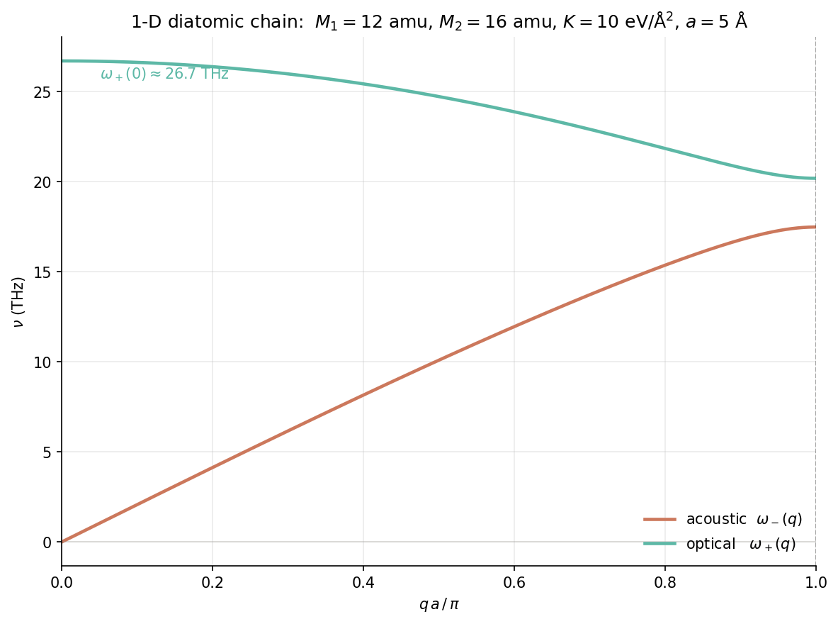
Figure 1. Phonon dispersion of a 1-D diatomic chain. The horizontal axis is the phonon wavevector $q$ in units of $\pi/a$ (the BZ boundary is at $q a / \pi = 1$). The vertical axis is the frequency in THz. The two branches are non-degenerate everywhere except at $q = 0$ (where the acoustic branch touches zero) and at the $\Gamma$ point of the acoustic zone, where the optical mode sits. The frequency gap at the BZ boundary is $\omega_+ - \omega_- \approx 3.7$ THz, in agreement with the analytical expression \eqref{eq:ch-10-worked-gap}.

The relevant code is reproduced below; the script is the source of truth.

# dft_notes/python_codes/chapter_10/01-diatomic-chain.py
import os
import numpy as np
import matplotlib

matplotlib.use("Agg")  # headless - no display required
import matplotlib.pyplot as plt

M1 = 12.0  # mass of atom 1, amu
M2 = 16.0  # mass of atom 2, amu
K  = 10.0  # force constant, eV/Å^2
A  = 5.0   # lattice constant, Å

eV_to_J   = 1.602176634e-19
A_to_m    = 1.0e-10
amu_to_kg = 1.66053906660e-27
THz_to_Hz = 1.0e12

K_SI  = K * eV_to_J / A_to_m ** 2
M1_SI = M1 * amu_to_kg
M2_SI = M2 * amu_to_kg

N_Q = 401
q_frac = np.linspace(0.0, 1.0, N_Q)
q_vals = q_frac * np.pi / A

sum_inv = 1.0 / M1_SI + 1.0 / M2_SI
inside = sum_inv ** 2 - 4.0 * np.sin(q_vals * A / 2.0) ** 2 / (M1_SI * M2_SI)
omega_sq_plus  = K_SI * (sum_inv + np.sqrt(inside))
omega_sq_minus = K_SI * (sum_inv - np.sqrt(inside))
nu_plus_THz  = np.sqrt(omega_sq_plus)  / (2.0 * np.pi) * 1.0e-12
nu_minus_THz = np.sqrt(omega_sq_minus) / (2.0 * np.pi) * 1.0e-12

fig, ax = plt.subplots(figsize=(8, 6))
ax.plot(q_frac, nu_minus_THz, color="#cc785c", lw=2.2,
        label=r"acoustic $\omega_-(q)$")
ax.plot(q_frac, nu_plus_THz,  color="#5db8a6", lw=2.2,
        label=r"optical  $\omega_+(q)$")
ax.axvline(1.0, color="#3d3d3a", lw=0.8, ls="--", alpha=0.5)
ax.set_xlabel(r"$q\, a\,/\,\pi$")
ax.set_ylabel(r"$\nu$ (THz)")
ax.set_title(r"1-D diatomic chain: $M_1 = 12$ amu, $M_2 = 16$ amu, "
             r"$K = 10$ eV/Å$^2$, $a = 5$ Å")
ax.legend(frameon=False, loc="lower right")
ax.grid(True, alpha=0.25)
ax.set_xlim(0.0, 1.0)
for spine in ("top", "right"):
    ax.spines[spine].set_visible(False)
fig.tight_layout()

here = os.path.dirname(os.path.abspath(__file__))
plots_dir = os.path.join(here, "plots")
os.makedirs(plots_dir, exist_ok=True)
out = os.path.join(plots_dir, "01-diatomic-chain.png")
fig.savefig(out, dpi=150, bbox_inches="tight")
print(f"Wrote {out}")

Note. The numerical values can be cross-checked with the analytical expressions of §10.9.4. At $q = 0$ the script returns the optical-branch frequency $\omega_+/(2\pi) = 26.7$ THz and the acoustic-branch frequency $\omega_- = 0$ — both in agreement with \eqref{eq:ch-10-worked-optic} and the limit $\omega_- \to v_s q$ as $q \to 0$. At $q = \pi/a$ the script returns $\omega_- = 17.5$ THz and $\omega_+ = 20.2$ THz, the two values given by $2K/M_1$ and $2K/M_2$ in the same units.

10.10 Workflow

The end-to-end workflow of a phonon calculation in the harmonic approximation is summarised below. The two main routes are frozen-phonon (top branch) and DFPT (bottom branch); they share the same starting geometry and the same output (the dispersion + DOS), but the intermediate steps differ.

%%{init: {'flowchart': {'htmlLabels': true, 'curve': 'basis'}}}%%
graph TD
  A["Relax geometry<br/>Hellmann-Feynman forces<br/>(ch. 09)"] --> B["Converged<br/>equilibrium cell<br/>(a, c, atomic positions)"]
  B --> C{"Choose method"}
  C -->|"frozen phonon"| D["Build supercell<br/>L1 x L2 x L3 primitive cells"]
  C -->|"DFPT"| E["Stay in primitive cell<br/>(unit cell of the perturbation)"]
  D --> F["Apply commensurate<br/>displacement pattern<br/>u_I = U e^{i q.R_I}"]
  E --> G["Solve Sternheimer<br/>equation for each<br/>q and branch s"]
  F --> H["SCF on supercell<br/>(N times, one per displacement)"]
  G --> H2["Self-consistent<br/>rho^(1) and psi_n^(1)"]
  H --> I["Fit force constants<br/>Phi(R) from forces"]
  H2 --> J["Compute force constants<br/>from 2n+1 formula"]
  I --> K["Fourier transform<br/>Phi(R) to D(q)"]
  J --> K
  K --> L["Diagonalise D(q)<br/>at each q"]
  L --> M["Phonon dispersion<br/>omega_s(q)"]
  M --> N["Phonon DOS g(omega)"]
  N --> O["Thermodynamic functions<br/>F(T), S(T), C_V(T)"]
  M --> P["Optional: e-ph coupling<br/>g_mn(q,k), alpha^2 F(omega)"]
  P --> Q["Superconducting T_c<br/>(McMillan / Eliashberg)"]

  classDef input fill:#eef0e6,stroke:#3a4031,color:#1c1f17;
  classDef step  fill:#d6dcc8,stroke:#3a4031,color:#1c1f17;
  classDef output fill:#cc785c,stroke:#1c1f17,color:#ffffff;
  class A input
  class B input
  class C step
  class D step
  class E step
  class F step
  class G step
  class H step
  class H2 step
  class I step
  class J step
  class K step
  class L step
  class N step
  class P step
  class M output
  class O output
  class Q output

The decision node `C{Choose method}’ is the one a practitioner spends the most time on. DFPT is preferred for primitive cells and for long-wavelength properties (LO–TO splitting, Born effective charges, the dielectric tensor). Frozen phonon is preferred for supercells (defects, alloys) and when DFPT is not available. The two routes converge to the same answer in the limit of a converged $\mathbf q$-mesh; the cost is just different.

10.11 Problems

10.12 What we left out

This chapter scratched the surface of phonon physics. Some of what we skipped:

• Phonon linewidths and anharmonic self-energies in detail. Equation \eqref{eq:ch-10-pp-width} is the second-order expression for the linewidth from cubic anharmonicity. The full anharmonic self-energy requires a self-consistent summation of diagrams (the “self-consistent phonon” or “renormalisation-group” approaches), and the fourth-order $E^{(4)}$ contributes both a frequency shift and a quartic broadening. We did not derive the full diagrammatic machinery; see Maradudin & Fein (1962) for the original treatment.
• The Allen–Heine–Cardona formalism in detail. Equation \eqref{eq:ch-10-ahc} is the zero-order (i.e. non-self- consistent) version of the AHC theory. The self-consistent version (sometimes called the “AHC-SC” or “cumulant” expansion) accounts for the renormalisation of the electronic states by the phonon self-energy, and gives quantitatively accurate band-gap renormalisations even in strongly anharmonic materials. The implementation in modern DFPT codes (Quantum ESPRESSO, ABINIT) is non-trivial and we did not give the formulas.
• Phonons in magnetic materials. In a magnetically ordered crystal (ferromagnet, antiferromagnet) the spin degrees of freedom couple to the lattice, and there are magnon–phonon hybrid modes. The spin–lattice coupling is a separate electron-phonon-like matrix element involving the spin density rather than the charge density, and is not covered by the formalism of §10.8. We did not treat it.
• Phonons at surfaces and interfaces. The translational symmetry of a surface or interface is broken in the direction normal to the surface, so the surface-phonon dispersion lives in a 2-D Brillouin zone and has additional modes (the Rayleigh surface acoustic wave, the Lucas modes, the Fuchs–Kliewer modes at surfaces of ionic crystals). The ab initio treatment follows the same DFPT recipe as for bulk, but the supercell must contain enough vacuum to isolate the two surfaces. We did not give the formulas.
• Phonon dynamics in real time. The harmonic approximation gives static normal modes. To describe real-time phonon dynamics (e.g. coherent-phonon experiments, phonon Boltzmann transport in the transient regime) one needs the time-dependent extension of the harmonic Hamiltonian, the phonon Boltzmann transport equation, or ab initio molecular dynamics. The state of the art is the non-equilibrium Green’s function (NEGF) treatment of phonons, which generalises the phonon self-energy to a $2 \times 2$ matrix in Keldysh space. We did not derive it.
• Phonon–photon coupling (polaritons). In an ionic crystal, the long-wavelength TO phonons couple to infrared photons through the macroscopic electric field, and the resulting polariton modes are hybrid phonon–photon excitations. The polariton dispersion is a textbook example of strong coupling between two bosonic modes, and is the foundation of infrared spectroscopy of solids. We did not give the polariton dispersion relation; see Kittel, Introduction to Solid State Physics chapter on optical processes.

Next: chapter 11 — Band structures: the electronic density of states, projected DOS, Fermi-surface topology, and the connection to transport.