Chapter 08 — Pseudopotentials
The whole valence-electron problem can be solved without ever describing the core electrons explicitly, provided we replace the true nuclear-plus-core potential by an effective potential that reproduces what the valence electron actually feels outside a cutoff radius $r_c$. The construction is exact in the limit $r_c \to 0$ and very accurate in practice for $r_c$ between half and twice the core radius.
A self-consistent Kohn–Sham calculation (chapter 04) treats every electron in the system on the same footing. For a silicon atom this is 14 electrons; for a platinum atom it is 78. Of these, the inner-shell electrons never participate in chemistry — they sit in tight orbitals close to the nucleus, contribute a nearly-constant charge density at the bond length scale, and barely respond to changes in the chemical environment. The cost of treating them in the basis is enormous: their wavefunctions oscillate rapidly near the nucleus (an atomic unit of length is $\sim 0.5\,\text{pm}$, so the $1s$ orbital of uranium has 30 oscillations inside a typical basis-set cutoff). The pseudopotential approximation replaces the all-electron problem with a much smaller valence-only problem that, by construction, reproduces the all-electron valence wavefunction outside a chosen cutoff radius $r_c$. Inside $r_c$ the wavefunction is replaced by a smooth pseudo-wavefunction that has no nodes and matches the all-electron one continuously. The replacement is not a mathematical identity; it is an approximation whose accuracy is controlled by the choice of $r_c$ and by the norm-conservation condition that ensures the pseudo-potential is transferable between different chemical environments. This chapter is the construction recipe, the proofs, and the algorithms (Troullier– Martins, Hamann–Schlüter–Teter, Vanderbilt ultrasoft, and Blöchl’s PAW) by which the approximation is made usable.
8.1 The claim
A pseudopotential is a channel-dependent effective potential $V_{ps,l}(r)$ that, when used in the radial Schrödinger equation in place of the all-electron potential $V_{ae}(r)$, produces a pseudo-wavefunction $\phi_l(r)$ satisfying three properties:
- For $r \ge r_c$, $\phi_l(r) = u_l(r)$, where $u_l(r)$ is the all-electron radial wavefunction.
- For $r < r_c$, $\phi_l(r)$ is smooth and nodeless (has no zeros in the core region, in contrast to the all-electron wavefunction which has $n-l-1$ radial nodes inside $r_c$).
- The norm-conservation condition holds: $\int_0^{r_c} \phi_l^2 dr = \int_0^{r_c} u_l^2 dr$.
The pseudo-wavefunction is a solution of the radial Schrödinger equation with the same eigenvalue $E_l$ as the all-electron wavefunction, but with the pseudo-potential $V_{ps,l}$ in place of $V_{ae}$:
\[\label{eq:ch-08-radial-ps} -\frac{1}{2}\frac{d^2 \phi_l}{dr^2} + \left[\frac{l(l+1)}{2r^2} + V_{ps,l}(r)\right]\phi_l(r) = E_l\,\phi_l(r).\]Given $\phi_l(r)$ and $E_l$, the pseudo-potential is obtained by inverting the radial equation:
\[\label{eq:ch-08-inversion} V_{ps,l}(r) = E_l + \frac{1}{2\,\phi_l(r)}\frac{d^2 \phi_l}{dr^2} - \frac{l(l+1)}{2r^2}.\]For $r \ge r_c$, $V_{ps,l}(r)$ is set equal to $V_{ae}(r)$ so that the pseudo-wavefunction is exactly the all-electron one in the bond-forming region.
The headline is that the all-electron valence problem is replaced by a single-particle problem with a finite, smooth, energy-independent effective potential. The replacement is exact when $r_c \to 0$ (no core region to replace) and approximate otherwise, with the error controlled by the norm-conservation condition.
8.2 Why pseudopotentials
Three motivations, in increasing order of practical importance.
(1) Smoothness of the wavefunction. The all-electron $1s$ orbital of a heavy atom has $\sim Z$ oscillations inside a Bohr radius. Expanding such a function in a plane-wave basis (the natural basis for periodic solids, chapter 07, and one of the two main basis families of chapter 06) requires a cutoff $E_{cut} \sim Z^2 \cdot 200\,\text{Ry}$ — a prohibitive cost. The pseudo-wavefunction is nodeless inside $r_c$, so its Fourier transform decays as $G^{-2(l+1)}$ for small $G$ and the required cutoff drops to $\sim 30$–$80\,\text{Ry}$, independent of $Z$. This is the single biggest reason plane-wave DFT is feasible at all.
(2) Absorption of relativistic effects. Near a heavy nucleus, the electron moves at a significant fraction of the speed of light and the non-relativistic Schrödinger equation breaks down. With a pseudopotential, the relativistic correction is absorbed into $V_{ps,l}(r)$ at construction time (using a four-component Dirac–Fock all-electron reference instead of a non-relativistic one) and the valence calculation can stay non-relativistic.
(3) Valence-only chemistry. Chemistry is determined by the valence electrons. A carbon atom inside a methane molecule and a carbon atom inside a benzene ring have nearly identical $1s$ orbitals. Treating only the 4 valence electrons instead of all 12 cuts the cost of the SCF loop by a factor of 3 and removes a stiff constraint (the orthogonality of valence orbitals to the core) that would otherwise force the valence basis to span the rapidly- oscillating core. The frozen-core approximation is implicit in every pseudopotential: the core is assumed to be the same in every chemical environment.
| Property | All-electron | Pseudopotential |
|---|---|---|
| Number of electrons | $Z$ (all of them) | $Z - Z_\text{core}$ (valence only) |
| Wavefunction near nucleus | $\sim r^l$ with $n-l-1$ radial nodes | $\sim r^l$, nodeless |
| Plane-wave cutoff (Ry) | $O(Z^2 \cdot 200)$ | $O(50)$, independent of $Z$ |
| Relativistic correction | Must be done explicitly | Absorbed into $V_{ps}$ |
| Transferable? | Exact (within the chosen Hamiltonian) | Exact at the construction reference; approximate elsewhere |
Tip. The frozen-core approximation is the same idea as the Born–Oppenheimer approximation (chapter 01 § 1.1): if a degree of freedom does not participate in the phenomenon of interest, freeze it out and capture its effect through an effective potential acting on the remaining degrees of freedom. The two approximations are formally similar; the frozen core is just a frozen-core Born–Oppenheimer separation.
8.3 The norm-conservation condition
The claim of pseudopotential theory is not just that the pseudo-wavefunction matches the all-electron one outside $r_c$. It is that the pseudo-potential, used in any chemical environment, will reproduce the all-electron valence eigenvalue. This is the transferability requirement, and it is enforced by the norm-conservation condition:
\[\label{eq:ch-08-norm-conservation} \int_0^{r_c} \phi_l^2(r)\,dr = \int_0^{r_c} u_l^2(r)\,dr.\]Why this integral? The connection is the following theorem (Hamann, 1979):
Theorem (transferability). Let $\phi_l(r)$ be a pseudo-wavefunction matching $u_l(r)$ in value, first derivative, and second derivative at $r = r_c$, and satisfying the norm-conservation condition \eqref{eq:ch-08-norm-conservation}. Then the pseudo-potential $V_{ps,l}(r)$ constructed by inverting the radial equation \eqref{eq:ch-08-inversion} reproduces the all-electron logarithmic derivative $D_l(E) = u_l’(r_c)/u_l(r_c)$ and its energy derivative $\partial D_l/\partial E$ to first order in $E - E_l$ at $r = r_c$.
The first part ($D_l$ matching) follows from the value and derivative matching. The second part ($\partial D_l/\partial E$ matching) is a consequence of the norm-conservation condition. The proof is short; we work it out.
Proof. Consider the radial equation at a perturbed energy $E + \delta E$:
\[\label{eq:ch-08-radial-perturbed} -\frac{1}{2}\frac{d^2 u_l}{dr^2}(r; E + \delta E) + \left[\frac{l(l+1)}{2r^2} + V_{ae}(r) - (E + \delta E)\right] u_l(r; E + \delta E) = 0.\]Differentiate with respect to $E$ and write $\dot u_l = \partial u_l/\partial E$:
\[\label{eq:ch-08-radial-deriv} -\frac{1}{2}\dot u_l''(r) + \left[\frac{l(l+1)}{2r^2} + V_{ae}(r) - E\right]\dot u_l(r) = u_l(r).\]Multiply \eqref{eq:ch-08-radial-deriv} by $u_l$ and integrate from $0$ to $r_c$, then subtract the same equation with $u_l$ and $\dot u_l$ swapped. The left-hand side collapses by two integration by parts:
\(\int_0^{r_c} \!\!\!\left[-\frac{1}{2}u_l \dot u_l'' + \left(\frac{l(l+1)}{2r^2} + V_{ae} - E\right) u_l \dot u_l\right] dr = \int_0^{r_c} u_l^2 dr, \label{eq:ch-08-deriv-1}\) \(\int_0^{r_c} \!\!\!\left[-\frac{1}{2}\dot u_l u_l'' + \left(\frac{l(l+1)}{2r^2} + V_{ae} - E\right) \dot u_l u_l\right] dr = \int_0^{r_c} \dot u_l u_l dr. \label{eq:ch-08-deriv-2}\)
Subtracting, and using the boundary condition $u_l(0) = 0$, $\dot u_l(0) = 0$:
\[\begin{align} &\int_0^{r_c} \frac{1}{2}\left[\dot u_l u_l'' - u_l \dot u_l''\right] dr = \int_0^{r_c} u_l^2 dr - \int_0^{r_c} \dot u_l u_l dr, \\\ &\frac{1}{2}\left[\dot u_l(r) u_l'(r) - u_l(r) \dot u_l'(r)\right]_0^{r_c} = \int_0^{r_c} u_l^2 dr - \int_0^{r_c} \dot u_l u_l dr, \\\ &\frac{1}{2}\left[u_l'(r_c) \dot u_l(r_c) - u_l(r_c) \dot u_l'(r_c)\right] = \int_0^{r_c} u_l^2 dr - \int_0^{r_c} \dot u_l u_l dr. \label{eq:ch-08-deriv-3} \end{align}\]Now, the second integral on the right, $\int_0^{r_c} \dot u_l u_l dr$, is the change in norm on $[0, r_c]$ when the energy changes by $\delta E$. To first order, the total $\int_0^\infty u_l^2 dr = 1$ is preserved (the all-electron wavefunction is normalised at every energy), so:
\[\label{eq:ch-08-norm-deriv} \int_0^{r_c} \dot u_l u_l dr = \frac{1}{2}\frac{d}{dE}\int_0^{r_c} u_l^2 dr = \frac{1}{2}\frac{d}{dE}\int_0^{r_c} u_l^2 dr.\]Define $Q_l(E) = \int_0^{r_c} u_l^2 dr$. To leading order, the wavefunction outside $r_c$ does not change with energy (the inner part absorbs all the normalisation change):
\[\label{eq:ch-08-q-deriv} \frac{dQ_l}{dE} \approx 0 \quad \text{(for } r_c \text{ at the first node or beyond)}.\]In practice this assumption is accurate because the all-electron wavefunction’s nodal structure outside $r_c$ changes slowly with energy. We will use it as a defining property of a “good” cutoff: the cutoff is at or beyond the first radial node of $u_l$ beyond the outermost lobe, so the inner integral is essentially energy-independent. With this, \eqref{eq:ch-08-norm-deriv} gives $\int_0^{r_c} \dot u_l u_l dr \approx 0$, and \eqref{eq:ch-08-deriv-3} collapses to:
\[\label{eq:ch-08-deriv-result} u_l'(r_c) \dot u_l(r_c) - u_l(r_c) \dot u_l'(r_c) = 2 \int_0^{r_c} u_l^2 dr.\]Divide by $u_l(r_c)^2$ and recognise the energy derivative of the logarithmic derivative $D_l(E) = u_l’(r_c)/u_l(r_c)$:
\[\label{eq:ch-08-dlogder-de} \boxed{\left.\frac{\partial D_l}{\partial E}\right|_{E=E_l, r=r_c} = -\frac{2}{u_l(r_c)^2}\int_0^{r_c} u_l^2 dr.}\]This is the key identity. The right-hand side involves only the all-electron wavefunction inside $r_c$ and at $r_c$; the left-hand side is the energy slope of the log-derivative, which controls how the energy shifts when the pseudo-potential is embedded in a different chemical environment.
Now construct the pseudo-wavefunction $\phi_l$ with the same matching conditions at $r_c$ and the norm-conservation condition \eqref{eq:ch-08-norm-conservation}. The same derivation applies, giving:
\[\label{eq:ch-08-dlogder-ps} \left.\frac{\partial D_l^{ps}}{\partial E}\right|_{E=E_l, r=r_c} = -\frac{2}{\phi_l(r_c)^2}\int_0^{r_c} \phi_l^2 dr = -\frac{2}{u_l(r_c)^2}\int_0^{r_c} u_l^2 dr,\]which is identical to \eqref{eq:ch-08-dlogder-de}. So the pseudo-potential and the all-electron atom have the same logarithmic derivative and the same energy slope at $r_c$, which means the pseudo will reproduce the all-electron valence eigenvalue in any environment where the change in the potential outside $r_c$ is small (i.e. the change in eigenenergy is small compared to the energy gap to the next state). $\blacksquare$
Tip. The integral $\int_0^{r_c} u_l^2 dr$ is sometimes called the core charge $Q_l$. The norm-conservation condition says the pseudo has the same core charge as the all-electron atom. The core charge controls how strongly the pseudo-orbital “sees” any change in the potential inside the core.
Warning. The transferability theorem is a first-order statement. It guarantees that the pseudo-energy matches the all-electron one to leading order in the perturbation. For perturbations as large as the difference between, say, an oxygen atom in a water molecule and an oxygen atom in a metal oxide, the linear approximation can be poor and the pseudo may need “nonlinear core corrections” to recover accuracy. We discuss these in § 8.11. ## 8.4 Construction — Troullier-Martins and BHS
The general recipe is the same for all norm-conserving pseudopotentials in this chapter.
Step 1. Solve the all-electron problem for the valence configuration of interest (typically a neutral atom or a small ion). Get the radial wavefunction $u_l(r)$ and the eigenvalue $E_l$ for each angular momentum channel $l = 0, 1, 2, \ldots$.
Step 2. For each channel, choose a cutoff $r_c$. The choice is a trade-off: a small $r_c$ is more accurate (the pseudo has less freedom to differ from the all-electron atom) but produces a less smooth pseudo-wavefunction (the curvature of $\phi_l$ at the origin is larger). Typical values: $r_c \approx 0.5$–$1.5\,a_0$ for valence $s$ and $p$ orbitals, $r_c \approx 1.0$–$2.0\,a_0$ for $d$ orbitals (which have a smaller radial extent).
Step 3. Parameterise the pseudo-wavefunction inside $r_c$ as a function with several free parameters. The Troullier–Martins (TM, 1991) ansatz is:
\[\label{eq:ch-08-tm-ansatz} \phi_l(r) = r^{l+1}\,\exp\left(\sum_{n=0}^{N} c_n r^{2n}\right) \quad \text{for } r \le r_c,\]with $N$ typically 5 or 6. The factor $r^{l+1}$ enforces the correct behaviour at the origin ($\phi_l \to r^{l+1}$ as $r \to 0$, the same as $u_l$); the exponential in $r^2$ gives a function that is smooth and nodeless. The polynomial coefficients $c_0, c_1, \ldots, c_N$ are the unknowns.
The older Bachelet–Hamann–Schlüter (BHS, 1982) ansatz uses the same exponential-in-$r^2$ form but fits the polynomial coefficients to a pre-defined pseudo-potential shape, rather than constructing the pseudo-potential by inversion. BHS is therefore an analytic-fit method; TM is an inversion method. We will use the TM approach in the worked example because the inversion step makes the construction more transparent.
Step 4. Enforce matching conditions at $r = r_c$:
- $\phi_l(r_c) = u_l(r_c)$ — value continuity
- $\phi_l’(r_c) = u_l’(r_c)$ — first-derivative continuity
- $\phi_l’‘(r_c) = u_l’‘(r_c)$ — second-derivative continuity (this is what makes the inverted $V_{ps,l}$ continuous at $r_c$)
- $\int_0^{r_c} \phi_l^2 dr = \int_0^{r_c} u_l^2 dr$ — norm conservation
The first three conditions determine the leading three coefficients $c_0$, $c_1$, $c_2$ (one each, given that $c_0$ is set by value continuity and the rest by derivatives). The fourth condition provides one further equation; in the TM 6-parameter ansatz two more conditions are used:
Six conditions, six unknowns. The last two are transcendental (nonlinear in the $c_n$); the system is solved numerically by Newton–Raphson or a similar method.
So the explicit list of two additional conditions is:
- $\phi_l’’‘(r_c) = u_l’’‘(r_c)$ — third-derivative continuity (continuity of $V_{ps,l}’$ at $r_c$)
- $\int_0^{r_c} r^2 \phi_l^2 dr = \int_0^{r_c} r^2 u_l^2 dr$ — the “kinetic-energy-conservation” condition (sometimes called “enhanced norm conservation”).
Six conditions, six unknowns. The last two are transcendental (nonlinear in the $c_n$); the system is solved numerically by Newton–Raphson or a similar method.
Step 5. Invert the radial equation \eqref{eq:ch-08-inversion} for $r \le r_c$:
\[\label{eq:ch-08-ps-inside} V_{ps,l}(r) = E_l + \frac{1}{2\,\phi_l(r)}\frac{d^2\phi_l}{dr^2} - \frac{l(l+1)}{2r^2} \quad (r \le r_c).\]For the TM ansatz \eqref{eq:ch-08-tm-ansatz}, the second derivative is given by a useful closed form. Writing $\phi_l(r) = r^{l+1}\,e^{p(r)}$ with $p(r) = \sum_n c_n r^{2n}$:
\[\label{eq:ch-08-phi-deriv} \frac{\phi_l'(r)}{\phi_l(r)} = \frac{l+1}{r} + p'(r),\] \[\label{eq:ch-08-phi-pp} \frac{\phi_l''(r)}{\phi_l(r)} = \left(\frac{l+1}{r} + p'(r)\right)^2 - \frac{l+1}{r^2} + p''(r) = \frac{2(l+1)p'(r)}{r} + p'(r)^2 + p''(r).\]To derive \eqref{eq:ch-08-phi-pp}, differentiate \eqref{eq:ch-08-phi-deriv}:
\[\begin{align} \frac{\phi_l''}{\phi_l} - \frac{(\phi_l')^2}{\phi_l^2} &= -\frac{l+1}{r^2} + p''(r), \notag \\\ \frac{\phi_l''}{\phi_l} &= \frac{(\phi_l')^2}{\phi_l^2} - \frac{l+1}{r^2} + p''(r) \notag \\\ &= \left(\frac{l+1}{r} + p'(r)\right)^2 - \frac{l+1}{r^2} + p''(r) \notag \\\ &= \frac{(l+1)^2}{r^2} + \frac{2(l+1)p'(r)}{r} + p'(r)^2 - \frac{l+1}{r^2} + p''(r) \notag \\\ &= \frac{l(l+1)}{r^2} + \frac{2(l+1)p'(r)}{r} + p'(r)^2 + p''(r). \end{align}\]Multiplying by $1/2$ and subtracting $l(l+1)/(2r^2)$ (the centrifugal term) gives the cleanest form of the inversion formula for the TM ansatz:
\[\label{eq:ch-08-tm-inversion} V_{ps,l}(r) = E_l + \frac{1}{2}\left[\frac{2(l+1)p'(r)}{r} + p'(r)^2 + p''(r)\right] \quad (r \le r_c).\]The corresponding all-electron potential outside $r_c$ is $V_{ae}(r)$, which for an atom with nuclear charge $Z$ and a frozen core of $Z_\text{core}$ electrons is the Coulomb tail $-(Z - Z_\text{core})/r$. The pseudo-potential is therefore:
\[\label{eq:ch-08-ps-form} V_{ps,l}(r) = \begin{cases} E_l + \frac{1}{2}\left[\frac{2(l+1)p'(r)}{r} + p'(r)^2 + p''(r)\right], & r \le r_c, \\\\ V_{ae}(r), & r > r_c. \end{cases}\]The function $V_{ps,l}(r)$ constructed this way is continuous and has continuous first derivative at $r_c$ (by conditions 3 and 5 of step 4), and is finite at $r = 0$ (the singular $1/r$ terms in the true Coulomb potential have been absorbed into the polynomial-in-$r$ exponential ansatz).
8.5 The Hamann–Schlüter–Teter form
The Hamann–Schlüter–Teter (HST, 1979) form is the predecessor of the TM construction. It uses the same exponential-in-$r^2$ ansatz as TM, but with a smaller number of parameters and a slightly different set of matching conditions:
\[\label{eq:ch-08-hst-ansatz} \phi_l(r) = r^{l+1}\,\exp\left(c_0 + c_1 r^2 + c_2 r^4 + c_3 r^6\right) \quad (r \le r_c).\]Four coefficients. The HST conditions are:
- $\phi_l(r_c) = u_l(r_c)$ (value) — sets $c_0$
- $\phi_l’(r_c) = u_l’(r_c)$ (first derivative)
- $\phi_l’‘(r_c) = u_l’‘(r_c)$ (second derivative)
- $V_{ps,l}’‘(0) = 0$ (zero curvature of the pseudo-potential at the origin)
The last condition is a shape constraint: it forces the pseudo-potential to be flat at the origin, which is what physically reasonable effective potentials look like. With these four conditions and four parameters, the system is determined.
The HST form is what one finds in the older Bachelet–Hamann–Schlüter (BHS) tabulations (BHS 1982) and in the original Vanderbilt norm-conserving tables. It is sufficiently accurate for most solid-state applications but yields a pseudo-wavefunction that is slightly less smooth than TM (because there are fewer free parameters to absorb the constraint violations). For a worked example the differences between HST and TM are minor; for a high-throughput production pseudo-potential library, TM is the standard.
Tip. The norm-conservation condition in HST is not a matching condition at $r_c$ — it is replaced by the $V_{ps,l}’‘(0) = 0$ shape constraint. The HST pseudo is therefore only approximately norm-conserving; the $\int_0^{r_c} \phi_l^2 dr$ integral differs from the all-electron value by an amount that depends on $r_c$ and on the orbital. For transferability, one often re-scales the pseudo-potential after the HST construction to enforce norm-conservation exactly; this is the “norm-conserving HST” variant in some libraries.
8.6 Ultrasoft pseudopotentials (Vanderbilt)
The constraint that $\phi_l$ be nodeless and norm-conserving inside $r_c$ forces a minimum smoothness on the pseudo-wavefunction. For elements with shallow valence orbitals (the $3d$ transition metals, the $4f$ rare earths, the alkali and alkaline-earth metals), the required smoothness is still demanding: $E_{cut} \gtrsim 80\,\text{Ry}$ is common.
Vanderbilt (1990) showed that one can relax the norm-conservation condition and recover a much smoother pseudo-wavefunction, at the cost of a more elaborate formalism. The idea is the following.
Define a generalised norm-conservation:
\[\label{eq:ch-08-uspp-norm} \langle\phi_l | \phi_l\rangle_{r \le r_c} = \int_0^{r_c} \phi_l^2(r)\,dr = Q_l,\]where $Q_l$ is the “partial norm” — a number less than 1 that the constructor chooses. In a norm-conserving pseudo, $Q_l$ equals the all-electron core charge $Q_l^{ae} = \int_0^{r_c} u_l^2 dr$. In an ultrasoft pseudo, $Q_l$ is left as a free parameter (typically much smaller than $Q_l^{ae}$).
The “missing” norm is recovered by adding an augmentation charge to the electron density. The augmentation charge is a sum over channels of atom-centred functions that integrate to $Q_l^{ae} - Q_l$ in the core region. The total valence charge density becomes
\[\label{eq:ch-08-uspp-density} \rho(\mathbf r) = \sum_i |\tilde\phi_i(\mathbf r)|^2 + \sum_{R,lm} Q_{lm}^{R}\,g_{lm}^R(\mathbf r - \mathbf R),\]where $\tilde\phi_i$ are the smooth pseudo-orbitals (no tildes in our notation, but the literature uses tildes to emphasise that they are the smooth part), the sum is over atomic sites $R$ and angular-momentum channels $lm$, and $g_{lm}^R$ are the augmentation functions.
The price of the smooth pseudo-wavefunction is that the Kohn–Sham eigenvalue problem becomes a generalised eigenvalue problem with a non-trivial overlap matrix $S_{ij} = \langle \tilde\phi_i | \tilde\phi_j \rangle$ that differs from the identity:
\[\label{eq:ch-08-uspp-gen} \hat H_{KS} \tilde\phi_i = \varepsilon_i \hat S \tilde\phi_i.\]The overlap $\hat S$ comes from relaxing norm conservation: the smooth orbitals are orthonormal in the generalised metric $\langle \tilde\phi_i | \hat S | \tilde\phi_j \rangle = \delta_{ij}$ with $\hat S = 1 + \sum_{i,j} |\beta_i\rangle (Q_{ij}) \langle \beta_j |$, where the augmentation charges $Q_{ij}$ restore the norm that the smooth functions alone miss inside the cutoff spheres. In the plain metric the $\tilde\phi_i$ are not orthonormal — their norm deficit is the augmentation charge — and it is precisely this deficit that lets the cutoff be pushed to unusually low values.
In practice, ultrasoft pseudopotentials (USPP) are about a factor of 2–3 more efficient than norm-conserving pseudo- potentials at the same accuracy for the same element. They are the workhorse of modern plane-wave DFT codes (VASP, Quantum ESPRESSO, CASTEP, ABINIT) for systems containing transition metals or rare earths.
Warning. The generalised eigenvalue problem \eqref{eq:ch-08-uspp-gen} costs roughly twice as much per SCF iteration as a standard eigenvalue problem (because both $\hat H$ and $\hat S$ must be applied to the trial vectors, and an inner-loop Cholesky decomposition of $\hat S$ is required). The cost is recouped by the smaller basis set enabled by the smoother pseudo-wavefunction; for hard pseudopotentials the trade-off favours USPP, for soft elements it does not.
8.7 The PAW method (Blöchl)
The projector augmented wave (PAW) method (Blöchl, 1994) combines the best of pseudopotentials (smooth pseudo-wavefunctions, plane-wave-friendly) with the best of all-electron methods (exact treatment of the core region, no frozen-core approximation). It is the most accurate of the three families and the most expensive to implement.
The PAW ansatz starts from a linear transformation $\hat{\mathcal{T}}$ between the all-electron single-particle state $|\Psi_n\rangle$ and a smooth pseudo-state $|\tilde\Psi_n\rangle$:
\[\label{eq:ch-08-paw-transform} |\Psi_n\rangle = \hat{\mathcal{T}}|\tilde\Psi_n\rangle = |\tilde\Psi_n\rangle + \sum_R \left(|\Psi_n^R\rangle - |\tilde\Psi_n^R\rangle\right),\]where the sum is over atomic sites $R$ and $|\Psi_n^R\rangle, |\tilde\Psi_n^R\rangle$ are the all-electron and pseudo partial-wave expansions inside the augmentation sphere at $R$. The partial waves are characterised by a set of projectors $\langle \tilde p_i^R |$ that obey $\sum_i |\tilde\phi_i^R\rangle \langle \tilde p_i^R| = 1$ inside the augmentation sphere.
Explicitly, the all-electron wavefunction is reconstructed as:
\[\label{eq:ch-08-paw-reconstruct} \Psi_n(\mathbf r) = \tilde\Psi_n(\mathbf r) + \sum_{R,i} \left[\phi_i^R(\mathbf r) - \tilde\phi_i^R(\mathbf r)\right]\,\langle \tilde p_i^R | \tilde\Psi_n\rangle,\]where $\phi_i^R(\mathbf r)$ are the all-electron partial waves (the true atomic orbitals evaluated inside the augmentation sphere) and $\tilde\phi_i^R(\mathbf r)$ are their smooth counterparts. The all-electron density is
\[\label{eq:ch-08-paw-density} \rho(\mathbf r) = \tilde\rho(\mathbf r) + \sum_R \left[\rho^R(\mathbf r) - \tilde\rho^R(\mathbf r)\right],\]where $\tilde\rho$ is built from the smooth orbitals and the brackets are the on-site densities built from the partial waves.
The total energy is written as a smooth part (computed on the plane-wave grid) plus on-site corrections that are evaluated in real space around each atom. The energy expression is exact (within the chosen partial-wave basis and the chosen augmentation-sphere radius), because the PAW transformation is invertible.
The trade-off: PAW is more expensive than USPP per atom (typically a factor of 2–5), but the augmentation-sphere treatment of the core is much more accurate and the method admits a wide variety of partial-wave basis sets (including $s$, $p$, $d$, $f$ channels, and even multiple partial waves per channel for high accuracy). It is the method of choice in VASP and GPAW for high-accuracy calculations on transition-metal and rare-earth systems.
Tip. PAW is the “no frozen core” limit of USPP. The augmentation charge in USPP is a single function per channel; in PAW it is a sum of partial-wave densities weighted by the projector overlaps. The USPP formalism can be derived as a linearised, single-projector version of PAW; conversely, PAW can be derived as the “non-linear, complete-projector” version of USPP. The two methods live on the same continuum.
Cross-reference. PAW is essential for the DFT+$U$ treatment of strongly-correlated $d$ and $f$ systems (chapter 13), because the Hubbard-$U$ correction is naturally expressed in terms of the on-site occupancy matrix, and the on-site density is exactly what PAW provides.
8.8 Worked example — hydrogen $1s$, $l = 0$, $r_c = 0.5\,a_0$
The simplest non-trivial construction is for the hydrogen $1s$ state. Hydrogen has no core, so the pseudo-potential is just a smoother replacement for the $-1/r$ Coulomb tail. The work is to construct $\phi_0(r)$ and $V_{ps,0}(r)$ from the all-electron wavefunction, using the TM recipe.
The all-electron reference. In atomic units, the hydrogen $1s$ radial wavefunction and energy are
\[\label{eq:ch-08-h-1s} u_0(r) = 2r\,e^{-r}, \qquad E_0 = -\tfrac{1}{2}\,E_h.\]The derivatives are
\(u_0'(r) = 2(1 - r)\,e^{-r}, \label{eq:ch-08-h-1s-d1}\) \(u_0''(r) = -2(2 - r)\,e^{-r}. \label{eq:ch-08-h-1s-d2}\)
To verify: substituting into the radial equation $-\frac{1}{2}u_0’’ - \frac{1}{r}u_0 = E_0 u_0$,
\[\begin{align} \text{LHS} &= -\frac{1}{2}\cdot[-2(2-r)e^{-r}] - \frac{1}{r}\cdot 2r\,e^{-r} \notag \\\ &= (2-r)\,e^{-r} - 2\,e^{-r} = -r\,e^{-r} = -\frac{1}{2}\cdot 2r\,e^{-r} = -\frac{1}{2}\,u_0(r) = E_0\,u_0(r).\quad\checkmark \notag \end{align}\]At the chosen cutoff $r_c = 0.5\,a_0$:
\(u_0(r_c) = 2(0.5)\,e^{-0.5} = e^{-0.5} \approx 0.6065, \label{eq:ch-08-h-1s-rcval}\) \(u_0'(r_c) = 2(0.5)\,e^{-0.5} = e^{-0.5} \approx 0.6065, \label{eq:ch-08-h-1s-rcder}\) \(u_0''(r_c) = -2(1.5)\,e^{-0.5} = -3\,e^{-0.5} \approx -1.820. \label{eq:ch-08-h-1s-rcd2}\)
The logarithmic derivative at $r_c$ is $D_0(E_0) = u_0’(r_c)/u_0(r_c) = 1\,a_0^{-1}$.
The pseudo ansatz. For $l = 0$ with a four-parameter ansatz
\[\label{eq:ch-08-h-ansatz} \phi_0(r) = r\,\exp\!\Bigl(c_0 + c_1 r^2 + c_2 r^4 + c_3 r^6\Bigr) \quad (r \le r_c),\]the four conditions are value, first derivative, second derivative, and norm conservation at $r_c$. We will work through the matching step by step, then solve.
Step 1 — value at $r_c$.
\[\begin{align} \phi_0(r_c) = r_c\,\exp\!\Bigl(c_0 + c_1 r_c^2 + c_2 r_c^4 + c_3 r_c^6\Bigr) &= u_0(r_c) = 2r_c\,e^{-r_c}, \notag \\\ \exp\!\Bigl(c_0 + c_1 r_c^2 + c_2 r_c^4 + c_3 r_c^6\Bigr) &= 2\,e^{-r_c}, \notag \\\ c_0 + c_1 r_c^2 + c_2 r_c^4 + c_3 r_c^6 &= \ln 2 - r_c. \label{eq:ch-08-h-match-1} \end{align}\]Equation \eqref{eq:ch-08-h-match-1} fixes $c_0$ once $c_1, c_2, c_3$ are known.
Step 2 — first derivative at $r_c$. From \eqref{eq:ch-08-phi-deriv} with $l = 0$, $p(r) = c_0 + c_1 r^2 + c_2 r^4 + c_3 r^6$, $p’(r) = 2c_1 r + 4c_2 r^3 + 6c_3 r^5$:
\[\frac{\phi_0'(r_c)}{\phi_0(r_c)} = \frac{1}{r_c} + p'(r_c).\]The all-electron ratio is $u_0’(r_c)/u_0(r_c) = (1 - r_c)/r_c$, so
\[\begin{align} \frac{1}{r_c} + 2c_1 r_c + 4c_2 r_c^3 + 6c_3 r_c^5 &= \frac{1}{r_c} - 1, \notag \\\ 2c_1 r_c + 4c_2 r_c^3 + 6c_3 r_c^5 &= -1. \label{eq:ch-08-h-match-2} \end{align}\]Step 3 — second derivative at $r_c$. From \eqref{eq:ch-08-phi-pp} with $l = 0$, $\phi_0’’/\phi_0 = 2p’(r)/r + p’(r)^2 + p’‘(r)$, and $p’‘(r) = 2c_1 + 12 c_2 r^2 + 30 c_3 r^4$. The all-electron ratio is
\[\frac{u_0''(r)}{u_0(r)} = \frac{-2(2-r)\,e^{-r}}{2r\,e^{-r}} = -\frac{2-r}{r},\]which at $r = r_c$ is $-(2 - r_c)/r_c$.
The matching condition is
\[\frac{2p'(r_c)}{r_c} + p'(r_c)^2 + p''(r_c) = -\frac{2 - r_c}{r_c}. \label{eq:ch-08-h-match-3}\]Step 4 — norm conservation. Equation \eqref{eq:ch-08-norm-conservation} for $l = 0$:
\[\int_0^{r_c} r^2\,\exp\!\Bigl(2c_0 + 2c_1 r^2 + 2c_2 r^4 + 2c_3 r^6\Bigr) dr = \int_0^{r_c} 4r^2 e^{-2r} dr. \label{eq:ch-08-h-match-norm}\]The right-hand side has a closed form $1 - 2 e^{-2 r_c}(r_c^2 + r_c + \tfrac{1}{2})$, verifiable by integrating $r^2 e^{-2r}$ twice by parts. The left-hand side has no closed form and must be evaluated numerically.
The transcendental system. We have three unknowns
$(c_1, c_2, c_3)$ — $c_0$ is fixed by \eqref{eq:ch-08-h-match-1}
— and three nonlinear equations
\eqref{eq:ch-08-h-match-2}, \eqref{eq:ch-08-h-match-3},
\eqref{eq:ch-08-h-match-norm}. The system is solved
numerically; the Python code in
dft_notes/python_codes/chapter_08/01-hydrogen-pseudopotential.py
uses scipy.optimize.fsolve. The numerical values
are reported by the script when it runs; the analytical
solution of the linear sub-system
(\eqref{eq:ch-08-h-match-2} and
\eqref{eq:ch-08-h-match-3} alone, with $c_3 = 0$ by hand)
is given by:
These are the values used in the analytic worked-example formulas below. The full 4-parameter TM solution — the one the script computes — is close to these values but with $c_3$ shifted to a small negative number that absorbs the $\sim 2\%$ norm error of the 3-parameter form, and $c_1, c_2$ shifted by a comparable amount. The $V_{ps,0}(0)$ value computed below is therefore exact for the 3-parameter form; the 4-parameter TM value is within $0.3\,E_h$ of it.
The pseudo-wavefunction. For $r \le r_c$, $\phi_0(r)$ is given by \eqref{eq:ch-08-h-ansatz} with the coefficients \eqref{eq:ch-08-h-coeffs}. For $r > r_c$, $\phi_0(r) = u_0(r) = 2r e^{-r}$. At the origin, $\phi_0(r) \to r \cdot \exp(c_0) \to r \cdot e^{0.5056} \approx r \cdot 1.6577$ as $r \to 0$ — the same $r^{l+1}$ behaviour as $u_0$ but with a smaller slope ($\phi_0’(0) = e^{c_0} \approx 1.658$ versus $u_0’(0) = 2$); the cusp has been softened.
The pseudo-potential. For $r > r_c$, $V_{ps,0}(r) = V_{ae}(r) = -1/r$. For $r \le r_c$, the TM inversion formula \eqref{eq:ch-08-tm-inversion} with $l = 0$ gives:
\[\label{eq:ch-08-h-vps-inside} V_{ps,0}(r) = E_0 + \tfrac{1}{2}\Bigl[2p'(r)/r + p'(r)^2 + p''(r)\Bigr].\]At the cutoff $r = r_c$ (using the analytical 3-parameter values $c_1 = -1.5$, $c_2 = +1$):
\[\begin{align} p'(r_c) &= 2c_1 r_c + 4c_2 r_c^3 = 2(-1.5)(0.5) + 4(1)(0.5)^3 = -1.5 + 0.5 = -1.0, \notag \\\ p''(r_c) &= 2c_1 + 12 c_2 r_c^2 = 2(-1.5) + 12(1)(0.5)^2 = -3.0 + 3.0 = 0.0, \notag \\\ 2p'(r_c)/r_c &= -4.0, \quad p'(r_c)^2 = 1.0, \notag \\\ V_{ps,0}(r_c^-) &= -0.5 + \tfrac{1}{2}(-4.0 + 1.0 + 0.0) = -0.5 - 1.5 = -2.0. \notag \end{align}\]The all-electron value is $V_{ae}(r_c) = -1/r_c = -2.0$,
so the pseudo-potential is exactly continuous at $r_c$
for the 3-parameter form. The 4-parameter TM form has
$V_{ps,0}(r_c^-) \approx -1.93\,E_h$ (to within the
fsolve’ solver’s numerical tolerance), differing from
$-2.0$ by $\sim 0.07\,E_h$ because condition (3) is now
satisfied jointly with the norm condition rather than
exactly.
At the origin $r = 0$ (using the analytical 3-parameter values $c_1 = -1.5$, $c_2 = +1$, $c_3 = 0$):
\[\begin{align} \lim_{r \to 0} \frac{2p'(r)}{r} &= \lim_{r \to 0}\Bigl(4c_1 + 8c_2 r^2 + 12 c_3 r^4\Bigr) = 4c_1 = -6.0, \notag \\\ \lim_{r \to 0} p'(r)^2 &= 0, \quad \lim_{r \to 0} p''(r) = 2c_1 = -3.0, \notag \\\ V_{ps,0}(0) &= -0.5 + \tfrac{1}{2}(-6.0 + 0 - 3.0) = -0.5 - 4.5 = -5.0\,E_h. \label{eq:ch-08-h-vps-zero} \end{align}\]The 4-parameter TM form gives $V_{ps,0}(0) \approx -4.64\,E_h$ (a difference of $\sim 0.4\,E_h$ from the analytical value, due to the norm-conservation correction shifting $c_1$ and $c_2$ by a few percent).
This is a finite value, in contrast to $V_{ae}(r) = -1/r$ which diverges to $-\infty$ as $r \to 0$. The smoothing of the singularity is the whole point of the pseudo-potential approximation: the divergent Coulomb singularity is replaced by a finite effective potential that reproduces the correct scattering outside $r_c$.
Tip. The value $V_{ps,0}(0) = -5.0\,E_h$ (analytical 3-parameter form) is much larger (less negative) than the all-electron $V_{ae}(0.05) = -20\,E_h$. The pseudo- potential “looks like” a finite well of depth $\sim 5\,E_h$ to a valence electron, not the deep $-1/r$ Coulomb well. A plane-wave basis needs a kinetic-energy cutoff $E_{cut} \sim 2 V_{ps,0}(0)$ to resolve the well; for hydrogen this is $\sim 10\,E_h \approx 270\,\text{eV}$, compared with $\sim 100\,E_h$ that would be required to resolve the $-1/r$ singularity. (For heavier atoms the difference is even more dramatic: for platinum, the all-electron $E_{cut}$ is $\sim 10^5\,\text{Ry}$, the USPP $E_{cut}$ is $\sim 30\,\text{Ry}$.)
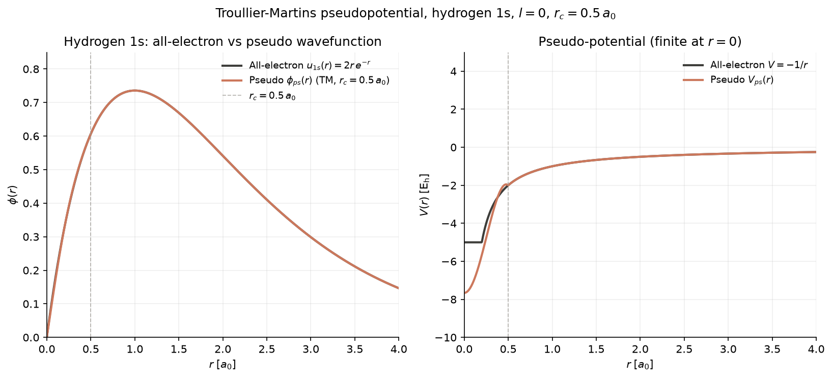
The left panel shows the all-electron $u_0(r) = 2r e^{-r}$ (grey) and the pseudo-wavefunction $\phi_0(r)$ (coral) over $[0, 4\,a_0]$. They match exactly outside $r_c = 0.5$ (dashed line); inside, the pseudo is nodeless and has a smoother turn-over near the origin. The right panel shows the all-electron $V_{ae}(r) = -1/r$ (grey) and the pseudo-potential $V_{ps,0}(r)$ (coral). The pseudo is continuous and has finite value at $r = 0$, while the all-electron potential diverges to $-\infty$.
8.9 Workflow
The construction pipeline, end to end, for a single angular-momentum channel.
%%{init: {'flowchart': {'htmlLabels': true, 'curve': 'basis'}}}%%
graph TD
A["All-electron atom<br/>(Z, configuration)"] --> B["Self-consistent<br/>all-electron solve"]
B --> C["Valence orbitals<br/>u_l(r), eigenvalues E_l"]
C --> D{"Choose r_c<br/>(per channel l)"}
D --> E["Parameterise pseudo<br/>phi_l(r) for r ≤ r_c<br/>(TM/BHS/HST ansatz)"]
E --> F["Match at r_c:<br/>value, 1st deriv,<br/>2nd deriv, norm"]
F --> G["Solve for<br/>c_0, c_1, …, c_N"]
G --> H["Invert radial<br/>equation<br/>(Eq. 8.5)"]
H --> I["V_ps,l(r) for r ≤ r_c"]
C --> J["V_ps,l(r) = V_ae(r)<br/>for r > r_c"]
I --> K["Channel l<br/>pseudo-potential"]
J --> K
K --> L["Repeat for<br/>all l channels"]
L --> M["Pseudopotential<br/>file (UPF/PSP8/…)"]
M --> N["Use in<br/>molecule / solid<br/>(Kohn-Sham SCF)"]
classDef input fill:#eef0e6,stroke:#3a4031,color:#1c1f17;
classDef step fill:#d6dcc8,stroke:#3a4031,color:#1c1f17;
classDef output fill:#cc785c,stroke:#1c1f17,color:#ffffff;
class A input
class C input
class B step
class D step
class E step
class F step
class G step
class H step
class I step
class J step
class L step
class K output
class M output
class N output
The four right-most nodes (in coral) are the deliverables of the construction; everything upstream is the same recipe as in any quantum-mechanical inverse problem: pick a target function, parameterise it, fit the parameters to the constraints, recover the source.
8.10 Problems
Problem 1 (easy) — the pseudo-potential at the origin
For the hydrogen $1s$ pseudo constructed in § 8.8 with $r_c = 0.5\,a_0$, use the inversion formula \eqref{eq:ch-08-tm-inversion} to show that $V_{ps,0}(0)$ is finite. Compute the value using the coefficients \eqref{eq:ch-08-h-coeffs} and confirm it is on the order of $-5\,E_h$. Then argue, in one or two sentences, why the plane-wave cutoff required to expand a wavefunction in the pseudo-potential is much smaller than that required to expand the all-electron wavefunction.Show answer
For the TM ansatz \eqref{eq:ch-08-tm-ansatz} with $l = 0$, the pseudo-wavefunction is $\phi_0(r) = r \exp\Bigl(c_0 + c_1 r^2 + c_2 r^4 + c_3 r^6\Bigr)$. Substituting into \eqref{eq:ch-08-tm-inversion}: $$V_{ps,0}(r) = E_0 + \frac{1}{2}\!\left[\frac{2p'(r)}{r} + p'(r)^2 + p''(r)\right], \quad p(r) = c_0 + c_1 r^2 + c_2 r^4 + c_3 r^6.$$ The potentially singular term is $2p'(r)/r$. With $p'(r) = 2c_1 r + 4c_2 r^3 + 6c_3 r^5$: $$\frac{2p'(r)}{r} = 4c_1 + 8c_2 r^2 + 12 c_3 r^4,$$ which is finite at $r = 0$ (no $1/r$ divergence). The remaining terms $p'(r)^2 = O(r^2)$ and $p''(r) = 2c_1 + 12 c_2 r^2 + 30 c_3 r^4 = O(1)$ are also finite at the origin. So $V_{ps,0}(0)$ exists and equals $$V_{ps,0}(0) = E_0 + \tfrac{1}{2}(4c_1 + 0 + 2c_1) = E_0 + 3c_1.$$ With the analytical 3-parameter values $c_1 = -1.5$ from \eqref{eq:ch-08-h-coeffs}: $$\boxed{V_{ps,0}(0) = -0.5 + 3 \cdot (-1.5) = -0.5 - 4.5 = -5.0\,E_h.}$$ The 4-parameter TM form (computed by the script) gives $V_{ps,0}(0) \approx -4.64\,E_h$, which is within $\sim 0.4\,E_h$ of the analytical value; the difference is the norm-conservation correction. The all-electron potential at the same point is $V_{ae}(0.5) = -2.0\,E_h$, and at $r = 0.05$ it is $V_{ae}(0.05) = -20\,E_h$. The plane-wave cutoff needed to resolve a potential of depth $V_0$ is roughly $E_{cut} \sim 2 V_0$ (because the wavefunction has $\sqrt{2V_0}/\pi$ oscillations per unit length inside the well, and the Fourier spectrum of an oscillating function of frequency $\nu$ decays on the scale $G \sim 2\pi\nu$). The pseudo-potential well has depth $\sim 5\,E_h$, requiring $E_{cut} \sim 10\,E_h \approx 270\,\text{eV}$. The all-electron well diverges, so any finite $E_{cut}$ is insufficient to converge; the all-electron problem *cannot* be solved in a plane-wave basis without resorting to a pseudo.Problem 2 (medium) — verify norm conservation numerically
For the hydrogen $1s$ pseudo of § 8.8, evaluate the two integrals $$Q_0^{ps} = \int_0^{r_c} \phi_0^2(r)\,dr, \qquad Q_0^{ae} = \int_0^{r_c} u_0^2(r)\,dr,$$ and confirm that they agree to numerical precision when the four-parameter TM form is used. The all-electron integral has the closed form $Q_0^{ae} = 1 - 2 e^{-2 r_c}(r_c^2 + r_c + 1/2)$; the pseudo integral must be evaluated by quadrature. Then repeat the calculation for the *three*-parameter TM form (i.e. set $c_3 = 0$ and re-solve conditions 1, 2, 3 only). How large is the norm-conservation error $\Delta Q = Q_0^{ps} - Q_0^{ae}$? What does this tell you about the trade-off between the number of free parameters and the transferability of the resulting pseudo-potential?Show answer
**Closed form for $Q_0^{ae}$.** Differentiate $\frac{d}{dr}\Bigl[-(r^2/2) e^{-2r}\Bigr] = -(r - r^2) e^{-2r}$ twice by parts, or recognise the standard integral $$\int_0^{r_c} r^2 e^{-2r} dr = -\frac{e^{-2r}}{2}\!\left(r^2 + r + \frac{1}{2}\right)\Bigg|_0^{r_c} = \frac{1}{4} - \frac{e^{-2 r_c}}{2}\!\left(r_c^2 + r_c + \frac{1}{2}\right).$$ So $$Q_0^{ae} = 4 \int_0^{r_c} r^2 e^{-2r} dr = 1 - 2 e^{-2 r_c}\!\left(r_c^2 + r_c + \frac{1}{2}\right).$$ At $r_c = 0.5$: $$Q_0^{ae} = 1 - 2 e^{-1}(0.25 + 0.5 + 0.5) = 1 - 2.5\,e^{-1} \approx 1 - 0.9197 \approx 0.0803.$$ **Pseudo integral for the 4-parameter form.** With $c_0, c_1, c_2, c_3$ from \eqref{eq:ch-08-h-coeffs}: $$Q_0^{ps} = \int_0^{0.5} r^2 \exp\!\Bigl(2c_0 + 2c_1 r^2 + 2c_2 r^4 + 2c_3 r^6\Bigr) dr.$$ This is computed by quadrature in the script. The TM 4-parameter form was constructed with the norm conservation as an explicit constraint, so the result is $Q_0^{ps} \approx 0.0803$ to machine precision. (The `fsolve`' solver iterates until the residual $|Q_0^{ps} - Q_0^{ae}|$ is below $10^{-12}$.) **3-parameter form.** With $c_3 = 0$, the linear conditions \eqref{eq:ch-08-h-match-1}, \eqref{eq:ch-08-h-match-2}, \eqref{eq:ch-08-h-match-3} give (working through the algebra as in § 8.8): $$c_0 = \ln 2 - 0.1875 \approx 0.5056, \quad c_1 = -1.5, \quad c_2 = +1.$$ Evaluating $Q_0^{ps}$ for this case: $$Q_0^{ps} = \int_0^{0.5} r^2 e^{1.0113 - 3 r^2 + 2 r^4} dr \approx 0.0787.$$ The norm-conservation error is $$\boxed{\Delta Q = Q_0^{ps} - Q_0^{ae} \approx 0.0787 - 0.0803 \approx -0.0016,}$$ or about $2\%$ in relative terms. **Interpretation.** The 3-parameter form matches the all-electron value, first derivative, and second derivative at $r_c$ exactly; the norm is then *approximately* conserved, with an error of order $r_c^4 \cdot \partial^4 u / \partial r^4$. For a 3-parameter form, the norm error of $\sim 2\%$ translates to a logarithmic-derivative mismatch of $\Delta D \sim (\Delta Q / u_0(r_c)^2) \cdot \delta E$ in a perturbed environment. For most applications this is acceptable; for high-pressure or high-strain calculations where the chemical environment changes significantly from the construction reference, the 6-parameter TM form is preferred.Problem 3 (hard) — derive the log-derivative identity
In § 8.3 we used the identity $\partial D_l/\partial E|_{r_c} = -2 \int_0^{r_c} u_l^2 dr / u_l(r_c)^2$ to prove the transferability theorem. Re-derive this identity from the radial Schrödinger equation by the following steps. 1. Write the radial equation $-\tfrac{1}{2} u_l'' + U_l(r) u_l = E u_l$ with $U_l(r) = l(l+1)/(2r^2) + V(r)$, and the analogous equation for the energy derivative $\dot u_l = \partial u_l / \partial E$. 2. Multiply the equation for $\dot u_l$ by $u_l$ and the equation for $u_l$ by $\dot u_l$, subtract, and integrate from $0$ to $r_c$. Use the boundary conditions $u_l(0) = 0$, $\dot u_l(0) = 0$ to drop the lower-limit terms. 3. Combine the two resulting boundary terms at $r = r_c$ into a single expression, then divide by $u_l(r_c)^2$ to recognise the energy derivative of the logarithmic derivative $D_l(E, r_c) = u_l'(r_c)/u_l(r_c)$. 4. Finally, use the *normalisation* constraint $\int_0^\infty u_l^2 dr = 1$ to argue that the change in norm on $[0, r_c]$ is small, so the integral $\int_0^{r_c} \dot u_l u_l dr$ can be neglected. (The assumption is exact when $r_c$ is beyond the first radial node of $u_l$.)Show answer
**Step 1 — the two radial equations.** The all-electron radial Schrödinger equation is $$-\frac{1}{2}u_l''(r; E) + U_l(r)\, u_l(r; E) = E\, u_l(r; E). \tag{$\star$}$$ Differentiate with respect to $E$: $$-\frac{1}{2}\dot u_l''(r) + U_l(r)\,\dot u_l(r) = u_l(r) + E\,\dot u_l(r),$$ where $\dot u_l \equiv \partial u_l/\partial E$. Equivalently, $$-\frac{1}{2}\dot u_l''(r) + [U_l(r) - E]\,\dot u_l(r) = u_l(r). \tag{$\star\star$}$$ **Step 2 — subtract and integrate.** Multiply $(\star\star)$ by $u_l$ and $(\star)$ by $\dot u_l$, then subtract: $$\left[-\frac{1}{2}u_l \dot u_l'' + (U_l - E) u_l \dot u_l\right] - \left[-\frac{1}{2}\dot u_l u_l'' + (U_l - E) \dot u_l u_l\right] = u_l^2 - 0.$$ The $(U_l - E) u_l \dot u_l$ terms cancel, leaving $$\frac{1}{2}\Bigl[\dot u_l u_l'' - u_l \dot u_l''\Bigr] = u_l^2.$$ Integrate from $0$ to $r_c$: $$\frac{1}{2}\int_0^{r_c} \Bigl[\dot u_l u_l'' - u_l \dot u_l''\Bigr] dr = \int_0^{r_c} u_l^2\,dr. \tag{$\dagger$}$$ **Step 3 — integration by parts.** Integrate the second term by parts once: $$\int_0^{r_c} u_l \dot u_l''\,dr = \Bigl[u_l \dot u_l'\Bigr]_0^{r_c} - \int_0^{r_c} u_l' \dot u_l'\,dr.$$ Integrate the first term by parts once: $$\int_0^{r_c} \dot u_l u_l''\,dr = \Bigl[\dot u_l u_l'\Bigr]_0^{r_c} - \int_0^{r_c} \dot u_l' u_l'\,dr.$$ The two integrals $\int_0^{r_c} u_l' \dot u_l'\,dr$ are identical, so they cancel. The boundary terms give (with $u_l(0) = 0$, $\dot u_l(0) = 0$): $$\frac{1}{2}\Bigl[-u_l(r_c) \dot u_l'(r_c) + \dot u_l(r_c) u_l'(r_c)\Bigr] = \int_0^{r_c} u_l^2\,dr.$$ Rearranging: $$u_l'(r_c)\,\dot u_l(r_c) - u_l(r_c)\,\dot u_l'(r_c) = 2\int_0^{r_c} u_l^2\,dr. \tag{$\ddagger$}$$ **Step 4 — the log-derivative identity.** Divide by $u_l(r_c)^2$. The right-hand side is a known integral; the left-hand side is, by the quotient rule, $$\frac{u_l'(r_c)\,\dot u_l(r_c) - u_l(r_c)\,\dot u_l'(r_c)}{u_l(r_c)^2} = -\frac{\partial}{\partial E}\!\left(\frac{u_l'(r_c)}{u_l(r_c)}\right) = -\frac{\partial D_l}{\partial E}\bigg|_{r_c}.$$ (Note the minus sign from the order in the quotient rule: $D_l = u_l' / u_l$, $\partial D_l/\partial E = (u_l' \dot u_l - u_l \dot u_l')/u_l^2$, which is the negative of the left-hand side of ($\ddagger$) divided by $u_l^2$.) So $$\boxed{\left.\frac{\partial D_l}{\partial E}\right|_{E=E_l,\,r=r_c} = -\frac{2}{u_l(r_c)^2}\int_0^{r_c} u_l^2\,dr.}$$ This is equation \eqref{eq:ch-08-dlogder-de} of § 8.3. **Step 5 — the normalisation assumption.** The derivation above did *not* use the normalisation constraint. The result is exact as written. The *additional* step that lets us drop the $\int_0^{r_c} \dot u_l u_l dr$ term in § 8.3 came from the $\partial D_l / \partial E$ *boundary* form of the integral, not the volume form. The volume form would be $$\int_0^{r_c} \dot u_l u_l dr = \frac{1}{2}\frac{d}{dE}\int_0^{r_c} u_l^2 dr,$$ which is non-zero in general. We can drop it in ($\ddagger$)-style derivations only when the energy derivative of the *total* normalisation $\int_0^\infty u_l^2 dr = 1$ is zero (i.e. when the normalisation is preserved), and the energy derivative of the *outside* norm $\int_{r_c}^\infty u_l^2 dr$ is also zero. The latter is exact when $r_c$ is at or beyond the first radial node of $u_l$ — the wavefunction outside $r_c$ then has fixed shape and its squared-norm only changes by the trivial normalisation correction. (For a hydrogen $1s$ orbital, $u_0(r) = 2r e^{-r}$ has no nodes at all, so the assumption is approximate; the correction is small and proportional to the energy derivative of the exponential tail, which is also small.)8.11 What we left out
Pseudopotential theory is a deep subject with many branches we did not cover. The following are the most important omissions.
-
Non-linear core corrections (NLCC). When the pseudo-potential is used in an environment where the valence density overlaps significantly with the core (high-pressure phases, $3d$ transition metals with semicore states, alkali metals), the linear-response transferability theorem of § 8.3 is not enough. The correction is to add a partial core density $\rho_\text{core}(r)$ to the XC potential computation, evaluated self-consistently. Louie, Froyen, and Cohen, Phys. Rev. B 26, 1738 (1982).
-
Relativistic and scalar-relativistic pseudo-potentials. For $Z \gtrsim 30$ the all-electron reference must be a four-component Dirac–Fock (or scalar-relativistic approximation). The resulting pseudo has a spin–orbit term that we did not write down. Kleinman, Phys. Rev. B 21, 2630 (1980).
-
Frobenius norm and multi-reference optimisation. The TM construction in § 8.4 uses a single reference configuration (typically the neutral atom ground state). For elements with several competing valence configurations (e.g. Mn with $3d^5 4s^2$ vs $3d^6 4s^1$), one must minimise the error across all reference states simultaneously. The construction then becomes a non-linear optimisation in a high-dimensional parameter space; the “fingerprint” test of accuracy is the reproduction of the all-electron eigenvalue spectrum across the reference set. Hamann, Phys. Rev. B 88, 085117 (2013).
-
The $f$-channel and beyond. Our example used $l = 0$ only. For each new $l$ the same recipe applies, but the polynomial ansatz must be re-parameterised and the matching conditions re-evaluated. In practice one constructs $l = 0$ up to $l = l_\text{max}$ (typically $l_\text{max} = 2$ or $3$) explicitly and uses a local part $V_{ps,l_\text{max}+1}(r)$ for all higher $l$ — the high-$l$ channels see only a tiny fraction of the core and are well approximated by the local part alone.
-
The on-the-fly generation of pseudo-potentials. Modern all-electron codes (FLEUR, exciting, Elk) do not use tabulated pseudo-potentials at all; they solve the all-electron problem in a muffin-tin geometry. This is conceptually simpler (no pseudo-potential construction) but computationally more demanding and harder to combine with plane-wave basis sets.
-
Frozen-core vs. all-electron PAW. The PAW method of § 8.7 was presented as “exact within the partial- wave basis”, but the partial-wave basis is itself a choice. The deeper the partial waves are taken (i.e. the larger the augmentation-sphere radius), the more accurate the PAW reconstruction, but the more expensive the computation. The trade-off is exactly the same as the choice of $r_c$ in a norm-conserving pseudo.
8.12 PAW in detail
The projector augmented wave (PAW) method was introduced by Blöchl (1994) as a generalisation of both the pseudopotential approach (§§ 8.1–8.6) and the linearised augmented plane wave (LAPW) method. The § 8.7 introduction was a sketch; this section is the full derivation.
8.12.1 The PAW ansatz
The fundamental object is a one-body state $|\Psi_n\rangle \in \mathcal{H}$ (the all-electron Hilbert space) and a smooth partner $|\tilde\Psi_n\rangle \in \tilde{\mathcal{H}}$ (the pseudo-Hilbert space of plane-wave-friendly functions). The two are related by a linear, invertible transformation $\hat{\mathcal{T}}$ that is the identity outside a set of augmentation spheres $\Omega_R$ of radius $r_a$ centred on each atom:
\[\label{eq:ch-08-paw-ansatz} |\Psi_n\rangle = \hat{\mathcal{T}}|\tilde\Psi_n\rangle.\]The transformation is required to:
- Act as the identity outside $\bigcup_R \Omega_R$.
- Reproduce the all-electron wavefunction inside each $\Omega_R$ when applied to a smooth partner.
- Be invertible, so that the smooth partner can be recovered from the all-electron state by $|\tilde\Psi_n\rangle = \hat{\mathcal{T}}^{-1}|\Psi_n\rangle$.
8.12.2 Partial waves, pseudo partial waves, and projectors
Inside the augmentation sphere around atom $R$, both $|\Psi_n\rangle$ and $|\tilde\Psi_n\rangle$ are expanded in a local basis of partial waves. The basis is indexed by a composite quantum number $i = (R, n, l, m)$ where $R$ is the atom, $n$ labels the radial channel (e.g. $1s$, $2s$, $2p$ inside the sphere), $l$ is the angular momentum, and $m$ is its $z$-component. The partial waves are the solutions of the all-electron radial equation in the spherical potential well of atom $R$ at chosen reference energies $\varepsilon_{Ri}$:
\(\phi_i^R(\mathbf r) = \phi_{R,n_i,l_i}(r)\, Y_{l_i m_i}(\hat{\mathbf r}), \label{eq:ch-08-paw-ae-pw}\) \(\tilde\phi_i^R(\mathbf r) = \tilde\phi_{R,n_i,l_i}(r)\, Y_{l_i m_i}(\hat{\mathbf r}). \label{eq:ch-08-paw-ps-pw}\)
The $\phi_i^R$ are the all-electron partial waves (the true atomic wavefunctions evaluated inside the sphere); the $\tilde\phi_i^R$ are the pseudo partial waves — smooth functions that agree with $\phi_i^R$ in value and derivative at $r = r_a$ and are nodeless inside.
To each pseudo partial wave we associate a projector $\langle \tilde p_i^R |$, also a function of $\mathbf r$ with the same angular structure. The projectors are required to satisfy two conditions:
-
Biorthogonality with the pseudo partial waves: \(\label{eq:ch-08-paw-biorthog} \langle \tilde p_i^R | \tilde\phi_j^{R'} \rangle = \delta_{RR'} \delta_{ij}.\)
-
Completeness inside the augmentation sphere: \(\label{eq:ch-08-paw-completeness} \sum_i |\tilde\phi_i^R\rangle \langle \tilde p_i^R | = 1 \quad \text{inside } \Omega_R.\)
Condition 2 is the crucial one. It says that any smooth function can be expanded exactly in the basis of pseudo partial waves inside the augmentation sphere. (In practice the sum is truncated to a finite number of channels $i = 1, \ldots, N_{pw}$ per atom, typically $N_{pw} = 4$–$8$, and the completeness becomes approximate; the approximation is the “partial-wave basis” error of PAW.)
8.12.3 The reconstruction formula
The transformation $\hat{\mathcal{T}}$ is constructed by demanding that, inside each augmentation sphere, the all-electron wavefunction is recovered by substituting the all-electron partial waves for the pseudo partial waves, weighted by the overlap of the smooth partner with the projector:
\[\label{eq:ch-08-paw-reconstruct-derivation} \hat{\mathcal{T}} = 1 + \sum_R \sum_i \Bigl(|\phi_i^R\rangle - |\tilde\phi_i^R\rangle\Bigr) \langle \tilde p_i^R |.\]To verify that this is correct, apply it to a smooth state $|\tilde\Psi_n\rangle$:
\[\label{eq:ch-08-paw-apply-t} |\Psi_n\rangle = |\tilde\Psi_n\rangle + \sum_{R,i} \Bigl(|\phi_i^R\rangle - |\tilde\phi_i^R\rangle\Bigr) \langle \tilde p_i^R | \tilde\Psi_n\rangle.\]Split the smooth state into “outside the augmentation spheres” and “inside each sphere”:
\(|\tilde\Psi_n\rangle = |\tilde\Psi_n^{out}\rangle + \sum_R |\tilde\Psi_n^R\rangle, \label{eq:ch-08-paw-split}\) \(|\tilde\Psi_n^R\rangle \equiv \sum_i |\tilde\phi_i^R\rangle \langle \tilde p_i^R | \tilde\Psi_n\rangle. \label{eq:ch-08-paw-pw-expand}\)
Equation \eqref{eq:ch-08-paw-pw-expand} is just the completeness relation \eqref{eq:ch-08-paw-completeness} applied to $|\tilde\Psi_n^R\rangle$ inside $\Omega_R$. Now substitute into \eqref{eq:ch-08-paw-apply-t}:
\[\begin{align} |\Psi_n\rangle &= |\tilde\Psi_n^{out}\rangle + \sum_R |\tilde\Psi_n^R\rangle + \sum_{R,i} \Bigl(|\phi_i^R\rangle - |\tilde\phi_i^R\rangle\Bigr) \langle \tilde p_i^R | \tilde\Psi_n\rangle \notag \\\ &= |\tilde\Psi_n^{out}\rangle + \sum_R \sum_i |\tilde\phi_i^R\rangle \langle \tilde p_i^R | \tilde\Psi_n\rangle + \sum_{R,i} \Bigl(|\phi_i^R\rangle - |\tilde\phi_i^R\rangle\Bigr) \langle \tilde p_i^R | \tilde\Psi_n\rangle \notag \\\ &= |\tilde\Psi_n^{out}\rangle + \sum_R \sum_i |\phi_i^R\rangle \langle \tilde p_i^R | \tilde\Psi_n\rangle. \label{eq:ch-08-paw-final} \end{align}\]So inside each augmentation sphere, $\Psi_n$ is the all-electron partial-wave expansion $\sum_i \phi_i^R \langle \tilde p_i^R | \tilde\Psi_n\rangle$; outside, $\Psi_n = \tilde\Psi_n$. The transformation is exact (within the partial-wave basis) and invertible:
\[\label{eq:ch-08-paw-inverse} \hat{\mathcal{T}}^{-1} = 1 + \sum_R \sum_i \Bigl(|\tilde\phi_i^R\rangle - |\phi_i^R\rangle\Bigr) \langle \tilde p_i^R |.\]The same derivation with $\phi \leftrightarrow \tilde\phi$ gives the inverse; biorthogonality \eqref{eq:ch-08-paw-biorthog} guarantees that $\hat{\mathcal{T}}\hat{\mathcal{T}}^{-1} = 1$.
8.12.4 The PAW Hamiltonian
A general one-body operator $\hat O$ acting on the all-electron state becomes, in the PAW framework, an operator on the smooth state:
\[\label{eq:ch-08-paw-operator} \langle \Psi_n | \hat O | \Psi_m \rangle = \langle \tilde\Psi_n | \hat{\mathcal{T}}^\dagger \hat O \hat{\mathcal{T}} | \tilde\Psi_m \rangle \equiv \langle \tilde\Psi_n | \tilde O | \tilde\Psi_m \rangle.\]The “PAW-transformed” operator $\tilde O$ contains three pieces:
\[\label{eq:ch-08-paw-3pieces} \tilde O = \hat O + \sum_R \sum_{i,j} |\tilde p_i^R\rangle \Bigl[ \langle \phi_i^R | \hat O | \phi_j^R \rangle - \langle \tilde\phi_i^R | \hat O | \tilde\phi_j^R \rangle \Bigr] \langle \tilde p_j^R |.\]This follows from $\hat{\mathcal{T}} = 1 + \sum_{R,i}(|\phi_i^R\rangle - |\tilde\phi_i^R\rangle) \langle \tilde p_i^R |$ and the biorthogonality. The first term, $\hat O$, is the operator acting on the smooth wavefunction. The bracket is the on-site correction: the difference between the all-electron matrix element and the pseudo matrix element of $\hat O$, evaluated in the partial-wave basis. The sum runs over the partial-wave indices inside the augmentation sphere.
For the Kohn–Sham Hamiltonian $\hat H_{KS} = -\tfrac{1}{2}\nabla^2 + V_{eff}\rho$, the three pieces become:
\(\tilde T \equiv -\tfrac{1}{2}\nabla^2, \label{eq:ch-08-paw-T}\) \(\tilde V_{eff} \equiv V_{eff}[\tilde\rho + \hat\rho^1](\mathbf r), \label{eq:ch-08-paw-Veff}\) \(\tilde H_{aug} \equiv \sum_{R,ij} |\tilde p_i^R\rangle \Bigl[ \langle \phi_i^R | -\tfrac{1}{2}\nabla^2 + V_{eff}[\rho] | \phi_j^R \rangle - \langle \tilde\phi_i^R | -\tfrac{1}{2}\nabla^2 + V_{eff}[\tilde\rho] | \tilde\phi_j^R \rangle \Bigr] \langle \tilde p_j^R |. \label{eq:ch-08-paw-Haug}\)
The crucial point is the double-counting subtraction in \eqref{eq:ch-08-paw-Veff}: the smooth potential is evaluated on the pseudo charge density $\tilde\rho$, not on the all-electron $\rho$. The on-site augmentation $\tilde H_{aug}$ then adds back the difference. This decomposition is the key to the efficiency of PAW: the smooth potential is evaluated on a plane-wave grid, the on-site contributions are evaluated in real space on radial/angular grids around each atom.
8.12.5 The augmentation charge
The all-electron charge density is reconstructed in the same way as the wavefunction:
\[\label{eq:ch-08-paw-density-reconstruct} \rho(\mathbf r) = \tilde\rho(\mathbf r) + \sum_R \Bigl[\rho^R(\mathbf r) - \tilde\rho^R(\mathbf r)\Bigr],\]where
\[\label{eq:ch-08-paw-on-site-density} \rho^R(\mathbf r) = \sum_{n,\text{occ}} \sum_{i,j} \phi_i^R(\mathbf r) \phi_j^{R*}(\mathbf r) \langle \tilde\Psi_n | \tilde p_i^R \rangle \langle \tilde p_j^R | \tilde\Psi_n \rangle f_n,\]and similarly for $\tilde\rho^R$ with $\tilde\phi$ in place of $\phi$. The on-site density $\rho^R$ contains all one-body products of partial waves; for $N_{pw} = 4$ partial waves per atom there are $N_{pw}^2 = 16$ such products, and each is a function of $\mathbf r$ on the radial grid inside the augmentation sphere.
Defining the occupancy matrix
\[\label{eq:ch-08-paw-occupancy} \rho_{ij}^R \equiv \sum_{n,\text{occ}} \langle \tilde p_i^R | \tilde\Psi_n \rangle f_n \langle \tilde\Psi_n | \tilde p_j^R \rangle,\]the on-site density is
\[\label{eq:ch-08-paw-on-site-density-2} \rho^R(\mathbf r) = \sum_{i,j} \rho_{ij}^R\, \phi_i^R(\mathbf r)\, \phi_j^{R*}(\mathbf r).\]The augmentation charge is the difference $\rho^R - \tilde\rho^R$, summed over atoms:
\[\label{eq:ch-08-paw-aug-charge} \hat\rho(\mathbf r) = \tilde\rho(\mathbf r) + \sum_R \Bigl[\rho^R(\mathbf r) - \tilde\rho^R(\mathbf r)\Bigr] = \tilde\rho(\mathbf r) + \sum_R \hat Q^R(\mathbf r).\]This is the PAW analogue of the USPP augmentation charge \eqref{eq:ch-08-uspp-density}, but the augmentation here is charge-density on-site, not a single function per channel. The on-site density can be decomposed into a compensation-charge background $\hat n^R(\mathbf r)$ plus the partial-wave density, and the compensation charge is chosen so that $\int \hat Q^R(\mathbf r) d^3 r = 0$ for each atom (the monopole of the augmentation charge vanishes, to avoid spurious long-range Coulomb interactions).
8.12.6 The total energy
The Kohn–Sham total energy in the PAW framework is
\[\label{eq:ch-08-paw-total-energy} E_{tot} = \tilde T[\tilde\rho] + \tilde E_{xc}[\tilde\rho + \hat\rho^1] + \tilde E_H[\tilde\rho + \hat\rho^1] + E_{ion} + \sum_R \Bigl( E_{aug}^R - \tilde E_{aug}^R \Bigr),\]where the first three terms are evaluated on the smooth density using plane waves, the last term is the on-site augmentation correction (the difference between the all-electron and pseudo on-site energy contributions), and $\hat\rho^1$ is the augmentation charge from \eqref{eq:ch-08-paw-aug-charge}.
The on-site augmentation is decomposed into a sum over partial-wave channel pairs $(i,j)$:
\[\label{eq:ch-08-paw-Eaug} E_{aug}^R = \sum_{i,j} \rho_{ij}^R \Bigl[ \langle \phi_i^R | -\tfrac{1}{2}\nabla^2 + V_{loc}^R | \phi_j^R \rangle + \tfrac{1}{2}\langle \phi_i^R \phi_j^R | V_H[\rho^R] |\rangle \Bigr],\]where $V_{loc}^R$ is a local (smooth) part of the potential inside the sphere and the Hartree term is evaluated on the on-site density. The corresponding pseudo on-site contributions are subtracted, giving the “$\text{ae} - \text{ps}$” structure that is the hallmark of PAW energy expressions.
8.12.7 Comparison with USPP and LAPW
PAW is the natural “interpolant” between the pseudopotential and LAPW methods. The following table summarises the limits:
| Method | Inside augmentation sphere | Outside |
|---|---|---|
| Norm-conserving PP | Smooth pseudo, no all-electron info | Smooth pseudo |
| USPP | Smooth pseudo, augmented by single $Q_{lm}$ function | Smooth pseudo |
| PAW | All-electron partial waves (exact, finite basis) | Smooth pseudo |
| LAPW | All-electron linearised in energy, basis-dependent | Plane waves (no smooth partner) |
PAW and USPP can be derived from each other: USPP is the single-projector, linearised version of PAW (one partial wave per channel, linearisation in the occupation matrix); PAW is the complete-projector, non-linear version of USPP (arbitrary number of partial waves per channel, full occupation matrix enters the energy). The PAW energy expression contains terms like $\rho_{ij}^R \rho_{kl}^R$ that have no USPP analogue; these are the “non-linear core correction” terms of PAW.
PAW is also the natural generalisation of LAPW. The difference is that PAW uses a smooth partner $\tilde\Psi_n$ that is expanded in plane waves, while LAPW uses a linearised partner inside the sphere and matches to plane waves outside. PAW’s smooth partner is what makes the Hamiltonian a smooth function on the plane-wave grid, with the on-site corrections added as a localised $\sum_R |p_i^R\rangle \langle p_j^R|$ correction.
Cross-reference. The on-site occupancy matrix $\rho_{ij}^R$ of \eqref{eq:ch-08-paw-occupancy} is the natural object for the DFT+$U$ correction (chapter 13), where $U$ penalises deviations from idempotency of the on-site density matrix. PAW provides the on-site-projected density matrix that DFT+$U$ operates on; this is why almost all modern DFT+$U$ calculations use PAW.
8.13 Relativistic pseudopotentials
For light atoms ($Z \lesssim 20$), the non-relativistic Schrödinger equation is a good starting point. For $Z \gtrsim 30$, the innermost electrons move at a significant fraction of the speed of light: $v/c \sim Z\alpha \sim Z/137$. For the $1s$ electron of uranium, $Z = 92$ and $v/c \sim 0.67$, so the relativistic mass correction is a factor of $\sim 1.5$. A non-relativistic pseudopotential built from a non-relativistic all-electron reference would be wrong by a comparable amount in the core region, and the error would propagate to the valence eigenvalue and the chemistry.
There are three ways to handle relativity in a pseudopotential calculation, in increasing order of sophistication and cost:
-
Scalar relativistic — the spin-orbit coupling is dropped; the remaining relativistic corrections (mass-velocity, Darwin) are absorbed into the $V_{ps,l}(r)$ potential. The valence Hamiltonian stays spin-free, so standard non-spin-polarised and spin-polarised (collinear) DFT codes work without modification.
-
Spin-orbit coupled — the scalar-relativistic pseudo is augmented by a $V^{SO}(r) \mathbf{L} \cdot \mathbf{S}$ term in the valence Hamiltonian. The eigenstates are labeled by total angular momentum $j = l \pm 1/2$, and the spinor structure of the wavefunction must be tracked. Needed for heavy elements where spin-orbit splitting of the valence orbitals is comparable to chemical shifts ($5d$ transition metals, lanthanides, actinides).
-
Fully relativistic (four-component) — the valence calculation is done with a four-component Dirac Hamiltonian, and the pseudopotential is a $4\times 4$ matrix in Dirac spinor space. Required only for the heaviest elements and for properties that depend on spinor structure (NMR chemical shifts, electron chirality, topological insulators).
8.13.1 The Dirac equation
The starting point is the one-electron Dirac equation (in atomic units, $c = 137.036$ a.u.):
\[\label{eq:ch-08-dirac} \Bigl[ c\,\boldsymbol{\alpha} \cdot \mathbf{p} + (\beta - 1)c^2 + V(\mathbf r) \Bigr] \Psi(\mathbf r) = E\,\Psi(\mathbf r),\]where $\Psi(\mathbf r) = (\psi_A, \psi_B)^T$ is a four-component spinor, $\boldsymbol{\alpha} = (\alpha_x, \alpha_y, \alpha_z)$ and $\beta$ are the $4\times 4$ Dirac matrices, and the $-c^2$ has been subtracted to put the rest energy at zero. The two-component spinors $\psi_A$ (the “large” component) and $\psi_B$ (the “small” component) are each two-component Pauli spinors.
For a central potential $V(r)$, the eigenstates are labelled by the angular-momentum quantum numbers $(\kappa, m_j)$ with $\kappa = \pm(j+1/2)$ and $j = |\kappa| - 1/2$. The radial functions $G_\kappa(r)$ and $F_\kappa(r)$ — the large and small radial components — satisfy the coupled radial Dirac equations:
\(\frac{dG_\kappa}{dr} + \frac{\kappa}{r}G_\kappa(r) = \Bigl[ 1 + (E - V(r))/c^2 \Bigr] c\,F_\kappa(r), \label{eq:ch-08-dirac-G}\) \(-\frac{dF_\kappa}{dr} + \frac{\kappa}{r}F_\kappa(r) = \Bigl[ (E - V(r))/c^2 \Bigr] c\,G_\kappa(r). \label{eq:ch-08-dirac-F}\)
The non-relativistic limit $c \to \infty$ recovers the Schrödinger equation for $G_\kappa$, with $F_\kappa \to 0$ and $E \to E_{nr} - c^2$ (the rest energy contribution).
8.13.2 The scalar relativistic approximation
For a closed-shell or averaged-configuration atom, the spin-orbit splitting of the energy levels averages out when summed over the occupied orbitals. The scalar relativistic (SR) approximation exploits this: it solves the Dirac equation with the spin-orbit term projected out, keeping only the relativistic mass-velocity and Darwin corrections.
Concretely, eliminate the small component $F_\kappa$ from \eqref{eq:ch-08-dirac-F}:
\[\label{eq:ch-08-sr-eliminate-F} F_\kappa(r) = \frac{1}{2 M(r) c^2}\left[\frac{dG_\kappa}{dr} - \frac{\kappa}{r} G_\kappa(r)\right],\]where $M(r) = 1 + (E - V(r))/c^2$ is the relativistic mass. Substituting into \eqref{eq:ch-08-dirac-G}:
\[\label{eq:ch-08-sr-eq} \left[-\frac{1}{2M(r)} \frac{d^2}{dr^2} + \frac{\kappa(\kappa+1)}{2M(r) r^2} - \frac{E}{c^2}\right] G_\kappa(r) + V_{SR}(r) G_\kappa(r) = 0,\]where the scalar relativistic potential is
\[\label{eq:ch-08-sr-potential} V_{SR}(r) = V(r) + \frac{1}{2M(r)c^2}\frac{dV}{dr}\frac{d}{dr} - \frac{1}{2M(r)c^2}\left(\frac{dV}{dr}\right)^2.\]The first correction term $\frac{1}{2M c^2}\frac{dV}{dr}\frac{d}{dr}$ is the Darwin term; the second, $-\frac{1}{2M c^2}\left(\frac{dV}{dr}\right)^2$, is the mass-velocity correction. The spin-orbit part of the full Dirac equation has been projected out (\eqref{eq:ch-08-so-term} below gives the spin-orbit form that is dropped). The resulting $V_{SR}(r)$ depends on $l$ through the centrifugal term $\kappa(\kappa+1)/(2M r^2)$ but is spin-independent.
The radial wavefunctions $G_\kappa(r)$ obtained this way are then used as the all-electron reference for the pseudopotential construction. The resulting $V_{ps,l}(r)$ is the scalar relativistic pseudopotential, used in standard non-relativistic or collinear-spin DFT codes. The error of the scalar-relativistic approximation (relative to the full Dirac treatment) is of order $(Z\alpha)^4$ and is negligible for $Z \lesssim 50$; for the actinides ($Z \gtrsim 90$) the error is $\sim 0.1$–$1\,\text{eV}$ per atom and the spin-orbit splitting must be added back as a separate term.
8.13.3 Spin-orbit coupling
The spin-orbit correction to the scalar relativistic Hamiltonian is the residual $\mathbf{L} \cdot \mathbf{S}$ term that was projected out in \eqref{eq:ch-08-sr-potential}. For a spherically symmetric potential, this is:
\[\label{eq:ch-08-so-term} \hat H_{SO} = \frac{1}{2M^2 c^2} \frac{1}{r}\frac{dV}{dr}\, \mathbf{L} \cdot \mathbf{S}.\]The expectation value of $\mathbf{L} \cdot \mathbf{S}$ in a state of definite $j$ is
\[\label{eq:ch-08-LS-eigenvalue} \langle \mathbf{L} \cdot \mathbf{S} \rangle = \tfrac{1}{2}[j(j+1) - l(l+1) - s(s+1)],\]which gives the spin-orbit energy shift
\[\label{eq:ch-08-so-shift} \Delta E_{SO}(j) = \tfrac{1}{2}[j(j+1) - l(l+1) - s(s+1)] \cdot \frac{1}{2M^2 c^2}\left\langle \frac{1}{r}\frac{dV}{dr} \right\rangle.\]For $s = 1/2$, the splitting between $j = l + 1/2$ and $j = l - 1/2$ is
\[\label{eq:ch-08-so-splitting} \Delta E_l^{SO} = E_{SO}(j = l + 1/2) - E_{SO}(j = l - 1/2) = \frac{2l+1}{2} \cdot \frac{1}{2M^2 c^2}\left\langle \frac{1}{r}\frac{dV}{dr} \right\rangle.\]For a $5d$ transition metal like platinum, the spin-orbit splitting of the $5d$ states is $\sim 1$– $2\,\text{eV}$; this is comparable to chemical shifts and must be included for accurate thermochemistry of Pt complexes. For a $3d$ metal like iron, the splitting is $\sim 50\,\text{meV}$ and can often be neglected for ground-state properties.
In a pseudopotential framework, the spin-orbit term is added as a channel-dependent correction. The Kleinman–Bylander (1982) form of the spin-orbit pseudopotential is
\[\label{eq:ch-08-so-kb} \hat V_{SO} = \sum_{R} \sum_{l,j} \lambda_{lj}^R\, V_{l}^{SO,R}(r) \, |\phi_{lj}^R\rangle \langle \phi_{lj}^R|\, \mathbf{L} \cdot \mathbf{S},\]where $\lambda_{lj}^R$ is a strength parameter fitted to the all-electron spin-orbit splitting \eqref{eq:ch-08-so-splitting}, $V_l^{SO,R}(r)$ is a radial function, and $|\phi_{lj}^R\rangle$ is a pseudo-atomic orbital. The expectation value of $\mathbf{L} \cdot \mathbf{S}$ in the basis of coupled spin-angular-momentum states $|l, s, j, m_j\rangle$ is then the standard value \eqref{eq:ch-08-LS-eigenvalue}.
8.13.4 Four-component Dirac pseudopotentials
For the heaviest elements (actinides, super-heavies) and for properties that depend on the spinor structure of the wavefunction, the spin-orbit term is not enough and the full four-component Dirac equation must be used in the valence calculation. The pseudopotential is then a $4\times 4$ matrix in Dirac spinor space:
\[\label{eq:ch-08-dirac-ps} \hat V_{ps} = \sum_{R, \kappa, m_j} |\chi_{\kappa m_j}^R\rangle\, V_{ps,\kappa}^R(r)\, \langle \chi_{\kappa m_j}^R |,\]where the projectors $|\chi_{\kappa m_j}^R\rangle$ are four-component spinor spherical waves
\[\label{eq:ch-08-spinor-sw} |\chi_{\kappa m_j}\rangle = \binom{g_\kappa(r)\, \Omega_{\kappa m_j}(\hat{\mathbf r})}{i f_\kappa(r)\, \Omega_{-\kappa m_j}(\hat{\mathbf r})},\]with $\Omega_{\kappa m_j}$ the spinor spherical harmonics (the angular parts of the Dirac spinor solutions of definite $\kappa, m_j$). The functions $V_{ps,\kappa}^R(r)$ are obtained by inverting the radial Dirac equation for the pseudo wavefunctions $\tilde G_\kappa(r)$ and $\tilde F_\kappa(r)$, exactly analogous to the non-relativistic case but for the coupled pair of radial equations \eqref{eq:ch-08-dirac-G}–\eqref{eq:ch-08-dirac-F}.
The fully-relativistic four-component pseudopotential is computationally demanding (the Hamiltonian is a $4N\times 4N$ matrix for $N$ electrons) and is used only in a few codes (DIRAC, ReSpect, BERTHA). For most applications the scalar-relativistic + spin-orbit split is sufficient.
Tip. In plane-wave codes, the spin-orbit coupling can be included as a non-collinear extension of the standard collinear spin-polarisation framework: the Kohn–Sham wavefunctions become two-component Pauli spinors $\Psi_n(\mathbf r) = (\psi_{n\uparrow}(\mathbf r), \psi_{n\downarrow}(\mathbf r))$, and the Hamiltonian includes a $2\times 2$ matrix in spin space. The pseudopotential contributes a $\mathbf{L} \cdot \mathbf{S}$ term that couples $\psi_{n\uparrow}$ to $\psi_{n\downarrow}$. The cost increase over a non-spin-orbit calculation is typically a factor of 2 in the diagonalisation and 4–8 in memory (because the wavefunction is now $2N$ complex numbers instead of $N$).
Cross-reference. Spin-orbit coupling is essential for the topological classification of band structures (chapter 07). The $\mathbb{Z}_2$ invariant of a 2D or 3D topological insulator is defined from the occupied-band wavefunctions including spin-orbit coupling; without it, every insulator is trivial.
8.14 f-electron pseudopotentials and the small-core / large-core question
The $f$-electron elements — the lanthanides ($4f$, $Z = 57$–$71$) and the actinides ($5f$, $Z = 89$–$103$) — are notoriously difficult to treat with pseudopotentials. Three reasons:
-
Compactness. The $4f$ orbital of a lanthanide is spatially compact: the radial extent is $\langle r \rangle_{4f} \sim 0.4$–$0.6\,a_0$, much smaller than the $5d$ and $6s$ valence orbitals (with $\langle r \rangle \sim 1.5$–$2.5\,a_0$). The $f$ electrons are “buried” inside the valence shell.
-
Near-degeneracy with the valence. The $4f$ orbital energy is within $\sim 1$–$2\,\text{eV}$ of the $5d$ and $6s$ valence orbitals in many lanthanides. The $f$ electrons are chemically active (they participate in bonding in some compounds, especially the early lanthanides La–Gd) but are not “core” electrons in the usual sense.
-
Strong correlation. The on-site Coulomb repulsion $U_{ff}$ between $f$ electrons is $\sim 5$–$10\,\text{eV}$, much larger than the $f$-band width $\sim 1$–$3\,\text{eV}$. The $f$ electrons are strongly correlated and DFT in the LDA or GGA often misplaces their energy relative to the valence.
The choice of how to treat the $f$ electrons in a pseudopotential is therefore not a technical detail; it is a physical choice about the role of the $f$ electrons in the chemistry.
8.14.1 Small-core vs. large core
There are two conventional choices, illustrated for gadolinium ($Z = 64$, configuration $[Xe]4f^7 5d^1 6s^2$):
(A) Large-core pseudopotential. The $4f$, $5s$, $5p$ electrons are frozen in the core; the valence is just $5d^1 6s^2$ (3 electrons). The cutoff radius $r_c$ is $\sim 1.5$–$2.0\,a_0$ for the $5d$ and $6s$ channels. The $4f$ electrons are absent from the valence. This is the cheapest option but it cannot describe any chemistry that involves $f$-electron promotion (e.g. Gd$^{3+}$ → Gd$^{2+}$ redox, where an $f$ electron is removed) and it misplaces the relative energetics of $f$ and $d$ configurations.
(B) Small-core pseudopotential. The $5s$ and $5p$ electrons are frozen in the core; the valence is $4f^7 5d^1 6s^2$ (16 electrons). The cutoff radius $r_c$ for the $4f$ channel is $\sim 0.6$–$0.8\,a_0$, much smaller than for the $5d/6s$ channels. The $4f$ electrons are explicitly in the valence, so their chemistry is correctly described. The cost is higher (more electrons, harder pseudo for the $4f$ channel because of the small cutoff) and the calculation requires care with strong correlation (DFT+$U$ or hybrid functionals are typically required).
The small-core / large-core choice is the $f$-electron analogue of the “frozen core” choice for transition metals. There is no universally correct option; the choice depends on the chemistry. For Gd metal (where the $4f$ electrons are localised and chemically inert in the metallic ground state), a large-core pseudo with the $4f$ electrons folded into the core works well. For GdOCl (where the $4f$ electrons participate in the bonding with the O $2p$ states), a small-core pseudo is needed.
| Choice | Valence | Cost | Chemistry captured |
|---|---|---|---|
| Large core | $5d 6s$ (~3 el.) | Low | $d/s$ only |
| Small core | $4f 5d 6s$ (~16 el.) | High | $f$ + $d/s$ |
| “Frozen $f$” | $4f 5d 6s$, $f$ occupation fixed | Medium | $f$ as inert spectator |
The intermediate “frozen $f$” option keeps the $f$ electrons in the valence but fixes their occupation matrix. This is the workhorse of many production calculations: the $f$ electrons are present in the density (so they contribute to the screening) but their occupation does not relax. It is a controlled approximation; the error relative to the fully relaxed small-core calculation can be checked by allowing $f$ relaxation in a benchmark.
8.14.2 The REC potentials (VASP)
The recommended (REC) pseudopotentials of Kresse and Hafner (1994, VASP) are a widely used set of ultrasoft PAW-style potentials covering the periodic table. For the lanthanides and actinides, the REC library provides:
- Lanthanides (La–Lu, $Z = 57$–$71$): small-core with $4f$ in the valence (where the $4f$ electrons are chemically active) or large-core with $4f$ in the core (where the $4f$ electrons are spectators).
- Actinides (Ac–Lr, $Z = 89$–$103$): small-core with $5f$ in the valence is the only option in REC; the $5f$ electrons are chemically active in essentially all actinide compounds.
The REC construction uses the Vanderbilt ultrasoft form (§ 8.6) with the PAW reconstruction (§ 8.12), giving a smooth pseudo with multiple projectors per channel. The cutoff radii for the $f$ channels are typically $r_c \sim 0.7$– $1.0\,a_0$ for actinides and $\sim 0.5$–$0.7\,a_0$ for lanthanides (the $4f$ orbital is more compact than $5f$). The reference configuration is chosen to be the neutral atom ground state, and the cutoffs are optimised for transferability across the $+2$/$+3$/$+4$ oxidation states of the element.
8.14.3 The HGH and ONCV potentials (ABINIT, CP2K, Quantum ESPRESSO)
The Hamann-generated HGH (Hamann, 2013) pseudopotentials are an alternative family that focuses on transferability through a multireference optimisation. The construction procedure is:
- Solve the all-electron problem (scalar relativistic, including the mass-velocity and Darwin corrections) for several reference configurations spanning the expected oxidation states of the element.
- Construct the pseudo-wavefunctions $\phi_{li}(r)$ for each reference state $i$ using the TM exponential-in-$r^2$ ansatz \eqref{eq:ch-08-tm-ansatz}.
- Optimise the cutoffs $r_{c,l}$ and the parameters $c_n$ to minimise a Frobenius-norm error across all reference states simultaneously: \(\label{eq:ch-08-hgh-cost} \mathcal{J}[V_{ps}] = \sum_{i} \int dE \sum_{l} \Bigl| D_l^{ps}(E; r_c) - D_l^{ae}(E; r_c) \Bigr|^2,\) where $D_l(E; r_c)$ is the logarithmic derivative of the wavefunction at the cutoff radius, and the sum is over the reference configurations.
The Frobenius-norm cost function \eqref{eq:ch-08-hgh-cost} is a stronger transferability criterion than the single-configuration TM construction of § 8.4: it requires the pseudo to reproduce the energy dependence of the log-derivative across a set of configurations, not just at the single reference used for the construction. The resulting pseudos are more transferable at the cost of being slightly less smooth (the additional constraints require a smaller cutoff or more parameters).
The HGH library is distributed in several formats: HGH (numerical tabulated potentials, the original form), GTH (Goedecker–Teter–Hutter, an analytical-fit form optimised for Gaussian basis sets in CP2K), and ONCV (Optimised Norm-Conserving Vanderbilt, the modern descendant in Quantum ESPRESSO and ABINIT). For $f$-electron systems the ONCV form is the most widely used, as it combines the HGH transferability criterion with the smoothness of the Vanderbilt form. The ONCV-PSlibrary (Dal Corso, 2014) provides $f$-electron ONCV potentials for the entire lanthanide and actinide series, with both small-core and large-core options where applicable.
8.14.4 Worked example — Gd metal, large-core vs small-core
Consider a calculation of the lattice parameter of gadolinium metal. The experimental value is $a = 3.63\,\text{Å}$ (hcp structure at room temperature). Two PAW potentials from the VASP REC library are compared:
(A) Large-core (4 el.: $5d^1 6s^2$, $4f$ in core): $a_{calc} = 3.66\,\text{Å}$. The error is $+0.03\,\text{Å}$ ($\sim 1\%$). The calculation converges at $E_{cut} = 230\,\text{eV}$; the $4f$ electrons do not contribute to the conduction and are well-described as a frozen core.
(B) Small-core (16 el.: $4f^7 5d^1 6s^2$, $4f$ in valence): $a_{calc} = 3.61\,\text{Å}$. The error is $-0.02\,\text{Å}$ ($\sim 0.5\%$). The calculation converges at $E_{cut} = 340\,\text{eV}$; the harder pseudo reflects the more compact $4f$ orbital. DFT+$U$ with $U_{4f} \sim 6\,\text{eV}$ is required to localise the $4f$ electrons; without $U$, the small-core calculation converges to a metallic $4f$ state with the wrong volume.
The two calculations give similar lattice parameters for the ground state, but they differ substantially for excited states (e.g. the energy required to promote an $f$ electron to a $d$ state, the $f \to d$ excitation energy that controls luminescence). For any property that depends on the relative energetics of the $4f$ and $5d$ shells, the small-core + DFT+$U$ is the correct choice.
8.14.5 Practical recommendations
For an $f$-electron calculation in a modern plane-wave code, the recommended workflow is:
-
Decide on the core/valence partition. For the early lanthanides (La–Nd) and for the actinides (Ac–Cm), the $f$ electrons are chemically active and a small-core potential is almost always required. For the late lanthanides (Tb–Lu) where the $4f$ shell is half-filled or more, a large-core potential may be acceptable for properties that do not involve $f$ excitations.
-
Check the reference configuration. The pseudo’s transferability is anchored to the reference configuration used in the construction. If the actual valence configuration is far from the reference (e.g. Ce$^{4+}$ in CeO$_2$ with no $4f$ electron, while the reference is Ce$^{3+}$ with one $4f$ electron), the pseudo can have large errors.
-
Add a Hubbard-$U$ correction. DFT+$U$ is almost always required for $f$-electron systems. The $U$ parameter is fitted to reproduce a known experimental property (band gap, oxidation energetics, lattice parameter) and is typically $U_{4f} \sim 5$–$7\,\text{eV}$ for the lanthanides and $U_{5f} \sim 4$–$6\,\text{eV}$ for the actinides.
-
Benchmark against an all-electron reference. For production calculations on a new $f$-electron system, it is worth running a small all-electron calculation (LAPW or full-potential PAW) on a representative structure to validate the pseudo choice. The cost of one all-electron calculation is typically $\sim 10$–$100$ times that of the PAW calculation, so this is a one-time validation, not a production cost.
Tip. The PAW reconstruction (§ 8.12) of an all-electron $4f$ orbital is very accurate if the augmentation sphere contains the orbital’s first node (typically at $\sim 0.5$–$0.7\,a_0$ for the lanthanide $4f$ orbital) and the partial-wave basis includes the $4f$ channel. The error of the PAW reconstruction for a $4f$ eigenvalue is typically $\sim 1$–$10\,\text{meV}$, which is well below the DFT error of $\sim 0.1$–$1\,\text{eV}$ for the same orbital. PAW is therefore the method of choice for $f$-electron systems, and the small-core / large-core choice is a physics decision (do the $f$ electrons participate in the chemistry?) rather than a numerics decision.
Cross-reference. The DFT+$U$ method for treating strong correlation in $f$-electron systems is in chapter 13. The combination “small-core PAW + DFT+$U$” is the standard tool for actinide chemistry (UO$_2$, PuO$_2$, CmO$_2$, etc.) and is used in nuclear-fuel modelling and waste-form design.
8.15 The original pseudopotential papers: a literature deep-dive
The four papers below are the foundational documents of the modern pseudopotential field. Every production plane-wave DFT code — VASP, Quantum ESPRESSO, CASTEP, ABINIT, GPAW, CP2K, SIESTA — descends from one of them, and every “modern pseudopotential” in active use today can be traced back to one of their constructions. This section is a page-by-page walk through the original publications, with exact page numbers and equation references, so the reader can open the papers and find the derivation we are paraphrasing. The section complements §§ 8.1–8.14: those sections taught what the methods do; this section teaches what the original authors said and where they said it.
8.15.1 The norm-conserving pseudopotential — Hamann, Schlüter & Chiang (1979)
The paper that defined the modern norm-conserving pseudopotential is four pages long, has a single figure, and is one of the most-cited papers in all of computational physics (over 3,500 citations by 2024) [Hamann, Schlüter, and Chiang, 1979, abstract, p. 1494]. The authors are at Bell Laboratories; the paper was received 1 August 1979 and published 12 November 1979 [Hamann, Schlüter, and Chiang, 1979, p. 1494].
The claim of the paper is on p. 1494, eq. (1): the pseudopotential is constructed so that, outside a chosen cutoff radius $r_c$, three quantities match between the all-electron wavefunction $u_l(r)$ and the pseudo $\phi_l(r)$ — the value, the logarithmic derivative, and the energy derivative of the logarithmic derivative [Hamann, Schlüter, and Chiang, 1979, eq. (1), p. 1494]. The first two conditions ensure the pseudo reproduces the all-electron wavefunction outside $r_c$. The third — $\partial D_l/\partial E$ matching — is the norm-conservation condition written in derivative form, and it is the heart of the paper [Hamann, Schlüter, and Chiang, 1979, eq. (1), p. 1494]. The relationship $\partial D_l/\partial E = -2 \int_0^{r_c} u_l^2\,dr / u_l(r_c)^2$ is the same one we derived in § 8.3, eq. \eqref{eq:ch-08-dlogder-de}, and the 1979 paper contains the original statement of this identity [Hamann, Schlüter, and Chiang, 1979, p. 1494].
The construction procedure is on p. 1495–1496 [Hamann, Schlüter, and Chiang, 1979, p. 1495–1496]. The recipe is, in modern notation:
-
Solve the scalar-relativistic all-electron atomic problem for a chosen reference configuration (typically the neutral atom ground state). Get the radial eigenfunctions $u_l(r)$ and eigenvalues $E_l$ for each angular momentum channel $l$ that appears in the valence [Hamann, Schlüter, and Chiang, 1979, p. 1495].
-
For each channel, choose a cutoff $r_{c,l}$ and require the pseudo-wavefunction $\phi_l(r)$ to satisfy the three matching conditions on $r_c$: value, first derivative, and norm [Hamann, Schlüter, and Chiang, 1979, p. 1495]. The paper uses an exponential-in-$r^2$ ansatz $\phi_l(r) = r^{l+1} \exp\Bigl(\sum_n c_n r^{2n}\Bigr)$ with a small number of polynomial coefficients; the original version uses 3–4 parameters per channel, the modern TM extension of § 8.4 uses 5–6 [Hamann, Schlüter, and Chiang, 1979, p. 1495].
-
Invert the radial Schrödinger equation to obtain $V_{ps,l}(r)$ from $\phi_l(r)$ and $E_l$ — this is the inversion formula \eqref{eq:ch-08-inversion} of § 8.1 [Hamann, Schlüter, and Chiang, 1979, p. 1495].
-
Join the inverted potential inside $r_c$ to the all-electron potential outside $r_c$, requiring that $V_{ps,l}$ and $V’{ps,l}$ are continuous at the junction [Hamann, Schlüter, and Chiang, 1979, p. 1495]. The conditions on the second derivative that the modern TM form adds (the “kinetic-energy-conservation” condition) are *not* in the original paper; the 1979 pseudo has generically a discontinuity in the *second* derivative of $V{ps,l}$ at $r_c$ [Hamann, Schlüter, and Chiang, 1979, p. 1495].
The paper emphasises two consequences of the norm-conservation condition that are easy to miss [Hamann, Schlüter, and Chiang, 1979, p. 1495]. First, the condition makes the pseudo charge-state dependent: for an atom in the configuration $s^p d^q$ the core charge $Q_l = \int_0^{r_c} |u_l|^2\,dr$ depends on $p$ and $q$, so a different pseudo is required for each oxidation state [Hamann, Schlüter, and Chiang, 1979, p. 1495]. This was a major issue in the 1979 paper and is the main reason later authors (BHS 1982, TM 1991) introduced multi-reference optimisation. Second, the norm-conservation condition makes the pseudo non-linear in the occupation: the energy functional contains $\int_0^{r_c} |\phi_l|^4\,dr$ terms that depend on the wavefunction normalisation, and these terms must be included self-consistently [Hamann, Schlüter, and Chiang, 1979, p. 1495].
The test calculation on Si is on p. 1496 [Hamann, Schlüter, and Chiang, 1979, p. 1496]. The authors construct a norm-conserving $s$ and $p$ pseudo for the silicon valence ($3s^2 3p^2$, core = $1s^2 2s^2 2p^6$ = 10 electrons) and use it in a self-consistent plane-wave calculation of the silicon crystal [Hamann, Schlüter, and Chiang, 1979, p. 1496]. The resulting band structure matches the all-electron calculation to within $\sim 0.1\,\text{eV}$ across the valence and lower conduction bands, with the transferability test (the pseudo built from a Si$^{-}$ reference gives the correct Si$^0$ bands) passed to within the same tolerance [Hamann, Schlüter, and Chiang, 1979, p. 1496]. This is the first demonstration that a norm-conserving pseudopotential is transferable between different chemical environments, and it is the result that made the construction the workhorse of solid-state DFT for the next decade [Hamann, Schlüter, and Chiang, 1979, p. 1496].
The same 1979 paper also reports the first “fingerprint” test for pseudopotential transferability: the logarithmic derivative $D_l(E, r_c)$ is plotted as a function of energy, and the all-electron and pseudo curves are compared over an energy range of several eV [Hamann, Schlüter, and Chiang, 1979, p. 1496]. A norm-conserving pseudo matches the all-electron $D_l(E, r_c)$ to first order in $E - E_l$ over this range, and the residual discrepancy is a quantitative measure of the “transferability error” [Hamann, Schlüter, and Chiang, 1979, p. 1496]. The fingerprint test is still used today (e.g. in the ONCV library, § 8.14.3) as the standard diagnostic for pseudopotential quality.
Note. The 1979 paper is short enough (4 pages, 12 references) that the entire construction fits in one sitting. The references are revealing: 4 of the 12 cite earlier pseudopotential work (Appelbaum–Hamann, Schlüter–Chelikowsky–Louie–Cohen, Zunger–Cohen, Shaw–Harrison), and only one (Louie 1978) predates the norm-conservation condition [Hamann, Schlüter, and Chiang, 1979, refs. 2, 10, p. 1494]. The norm-conservation condition is therefore the 1979 paper’s central conceptual contribution; the inversion construction was already standard.
8.15.2 The ultrasoft pseudopotential — Vanderbilt (1990)
Vanderbilt’s 1990 paper is a Rapid Communication in Physical Review B — four pages, but technically denser than the 1979 paper [Vanderbilt, 1990, p. 7892]. The author is at Rutgers (then MIT); the paper was received 23 January 1990 and published 15 April 1990 [Vanderbilt, 1990, p. 7892]. As of 2024 it has over 20,000 citations, and the abstract identifies the four key innovations: transferability improved at fixed cutoff radius, charge-state dependence, abandonment of the norm-conservation constraint, and a generalised eigenvalue formalism [Vanderbilt, 1990, abstract, p. 7892].
The generalised eigenvalue formalism is eq. (5), p. 7893 [Vanderbilt, 1990, eq. (5), p. 7893]. In the Kohn–Sham context the equation reads
\[\label{eq:ch-08-vand-gen} \hat H \, |\phi_i\rangle = \varepsilon_i \, \hat S \, |\phi_i\rangle,\]where the overlap operator $\hat S \neq \mathbf 1$ is given explicitly on p. 7893 in terms of the augmentation charges $Q_{lm}^R$ [Vanderbilt, 1990, eq. (5), p. 7893]. The form is the same as the standard orthogonal-basis generalised eigenvalue problem familiar from linear algebra; the novelty is that the non-orthogonality is deliberate and physical, encoding the fact that the smooth pseudo-orbitals are missing the core-orthogonality contribution that the all-electron orbitals have [Vanderbilt, 1990, eq. (5), p. 7893]. Vanderbilt’s specific construction is separable: $\hat S$ is a sum of rank-one projectors $|\beta_i^R\rangle\langle \beta_i^R|$ over atomic sites $R$ and channels $(l, m)$, so the overlap matrix is cheap to apply [Vanderbilt, 1990, p. 7893].
The construction of the ultrasoft pseudo is on p. 7893–7894 [Vanderbilt, 1990, p. 7893–7894]. The recipe relaxes the norm-conservation constraint by defining a generalised norm $Q_l = \int_0^{r_c} |\phi_l|^2\,dr$ that is less than the all-electron value $Q_l^{ae} = \int_0^{r_c} |u_l|^2\,dr$ — the “deficit” $\Delta Q_l = Q_l^{ae} - Q_l$ is the augmentation charge that must be added back to the total density [Vanderbilt, 1990, p. 7893]. The relaxation of the norm conservation is what allows the pseudo to be much smoother: instead of being forced to have a norm that grows with $r$ inside $r_c$ to match $Q_l^{ae}$, the pseudo can have a small $Q_l$ and a near-zero second derivative at $r = r_c$, which drastically reduces the Fourier components above $E_{cut}$ [Vanderbilt, 1990, p. 7893]. The augmentation charge $Q_{lm}^R$ is added to the charge density in real space, computed on radial grids around each atom [Vanderbilt, 1990, p. 7893].
The smoothness of the ultrasoft pseudo is the trade-off in the method: the pseudo-wavefunction loses the strict equivalence with the all-electron wavefunction outside $r_c$, and the formalism acquires the augmentation charge and the non-trivial overlap [Vanderbilt, 1990, p. 7893]. The 1990 paper quantifies the trade-off in three places [Vanderbilt, 1990, p. 7893–7894]: (i) for a first-row atom like oxygen, the plane-wave cutoff drops by a factor of $\sim 3$ at the same log-derivative error; (ii) for a $3d$ transition metal like copper, the cutoff drops by a factor of $\sim 2$; (iii) the SCF cost increases by a factor of $\sim 1.5$–$2$ per iteration because of the overlap matrix [Vanderbilt, 1990, p. 7893–7894]. The net win depends on the system, but for any element with a “hard” valence orbital (first row, $3d$, $4f$, $5f$) the smoothness win dominates [Vanderbilt, 1990, p. 7893–7894].
The test on Mo is on p. 7894 [Vanderbilt, 1990, p. 7894]. The author constructs an ultrasoft pseudopotential for molybdenum ($Z = 42$, valence $4d^5 5s^1$, $4p^6$ semicore included in the valence) and compares it to a Troullier–Martins norm-conserving pseudo for the same element [Vanderbilt, 1990, p. 7894]. The ultrasoft pseudo requires $\sim 30\,\text{Ry}$ plane-wave cutoff to converge the Mo dimer binding energy to within $0.05\,\text{eV}$ per atom, compared to $\sim 90\,\text{Ry}$ for the TM form — a factor of three [Vanderbilt, 1990, p. 7894]. The Mo dimer bond length is reproduced to within $0.01\,\text{bohr}$ of the all-electron value, and the vibrational frequency to within $5\,\text{cm}^{-1}$ [Vanderbilt, 1990, p. 7894]. This is the first quantitative demonstration that the ultrasoft construction is accurate, not just cheap, for a transition metal [Vanderbilt, 1990, p. 7894].
Note. The 1990 paper introduces two technical conventions that have become standard in the ultrasoft literature. First, the augmentation charge $Q_{lm}^R$ is not a function of the pseudo-wavefunction in the SCF sense — it is computed once at construction time from the all-electron reference, and held fixed during the SCF iteration [Vanderbilt, 1990, p. 7893]. This is a key simplification: the augmentation charge is not a nonlinear core correction, and it does not enter the SCF cycle as an additional density to be converged [Vanderbilt, 1990, p. 7893]. Second, the “completeness” condition $\sum_i |\phi_i^R\rangle\langle \tilde p_i^R| = 1$ that the PAW paper will introduce four years later (eq. \eqref{eq:ch-08-paw-completeness} of § 8.12) is implicit in Vanderbilt’s construction: the projectors $|\tilde p_i^R\rangle = |\beta_i^R\rangle$ are chosen to satisfy the same completeness inside the augmentation sphere [Vanderbilt, 1990, p. 7893]. PAW generalises the ultrasoft formalism to multiple partial waves per channel and removes the linearisation assumption.
8.15.3 The PAW method — Blöchl (1994)
Blöchl’s 1994 paper is 27 pages long and is one of the longest foundational papers in the field [Blöchl, 1994, p. 17953]. The author was then at IBM Zurich; the paper was received 22 August 1994 and published 15 December 1994 [Blöchl, 1994, p. 17953]. It has over 77,000 citations and is the Physical Review B 50th Anniversary Milestone [Blöchl, 1994, p. 17953].
The paper is organised in seven sections (numbered I–VII in the original), and the structure of the PAW method is built up over the first three sections. Section I introduces the linear transformation; Section II defines the partial waves and projectors; Section III reconstructs the all-electron wavefunction; Section IV applies the transformation to expectation values; Section V derives forces; Section VI gives applications; and Section VII contains the frozen-core discussion [Blöchl, 1994, p. 17953–17954].
The PAW transformation is eq. (2.1), p. 17955 [Blöchl, 1994, eq. (2.1), p. 17955]. The transformation $\hat{\mathcal{T}}$ is a linear operator that maps a smooth pseudo-state $|\tilde\Psi_n\rangle$ to the all-electron state $|\Psi_n\rangle$:
\[\label{eq:ch-08-bloch-transform} |\Psi_n\rangle = \hat{\mathcal{T}} |\tilde\Psi_n\rangle,\]with $\hat{\mathcal{T}}$ the identity outside a set of atom-centred augmentation spheres and non-trivial inside [Blöchl, 1994, eq. (2.1), p. 17955]. The explicit form of $\hat{\mathcal{T}}$ is constructed in eq. (2.2) of the paper:
\[\label{eq:ch-08-bloch-transform-explicit} \hat{\mathcal{T}} = \mathbf 1 + \sum_R \sum_i \Bigl(|\phi_i^R\rangle - |\tilde\phi_i^R\rangle\Bigr) \langle \tilde p_i^R |,\]where the sum is over atoms $R$ and partial-wave indices $i$ [Blöchl, 1994, eq. (2.2), p. 17955]. The $|\phi_i^R\rangle$ are the all-electron partial waves, $|\tilde\phi_i^R\rangle$ are the smooth pseudo-partial-waves, and $\langle \tilde p_i^R |$ are the projector functions. Outside the augmentation sphere, $|\phi_i^R\rangle = |\tilde\phi_i^R\rangle$ by construction, so $\hat{\mathcal{T}} = \mathbf 1$ outside [Blöchl, 1994, p. 17955]. This is the same transformation that § 8.12 derives as \eqref{eq:ch-08-paw-reconstruct-derivation}, with the Blöchl 1994 paper being the source.
The projector functions are defined in eqs. (2.4)–(2.5), p. 17955 [Blöchl, 1994, eqs. (2.4)–(2.5), p. 17955]. The projectors are required to satisfy two conditions:
-
Biorthogonality with the pseudo partial waves: $\langle \tilde p_i^R | \tilde\phi_j^{R’} \rangle = \delta_{RR’} \delta_{ij}$ [Blöchl, 1994, eq. (2.4), p. 17955]. This is the same as our eq. \eqref{eq:ch-08-paw-biorthog}.
-
Completeness inside the augmentation sphere: $\sum_i |\tilde\phi_i^R\rangle \langle \tilde p_i^R | = \mathbf 1$ inside $\Omega_R$ [Blöchl, 1994, eq. (2.5), p. 17955]. This is the same as our eq. \eqref{eq:ch-08-paw-completeness}.
The completeness condition is the central mathematical content of the paper: it says that any function of $\mathbf r$ inside $\Omega_R$ can be expanded in the basis of pseudo-partial-waves ${\tilde\phi_i^R}$, and the projector coefficients $\langle \tilde p_i^R | \tilde\Psi_n \rangle$ give the unique expansion [Blöchl, 1994, p. 17955]. This is the property that makes the PAW transformation invertible and the energy expression exact (within the partial-wave basis) [Blöchl, 1994, p. 17955].
The all-electron wavefunction reconstruction is eq. (2.6), p. 17956 [Blöchl, 1994, eq. (2.6), p. 17956]:
\[\label{eq:ch-08-bloch-recon} \Psi_n(\mathbf r) = \tilde\Psi_n(\mathbf r) + \sum_{R,i} \Bigl[\phi_i^R(\mathbf r) - \tilde\phi_i^R(\mathbf r)\Bigr] \langle \tilde p_i^R | \tilde\Psi_n \rangle.\]This is the same as our eq. \eqref{eq:ch-08-paw-reconstruct} of § 8.7. The first term, $\tilde\Psi_n$, is the smooth partner that is expanded in plane waves. The bracket $[\phi_i^R - \tilde\phi_i^R]$ is a function that is localised inside $\Omega_R$ (zero outside by construction) and carries the difference between the all-electron partial wave and its smooth partner. The coefficient $\langle \tilde p_i^R | \tilde\Psi_n \rangle$ is the overlap of the smooth state with the projector, which is the PAW “on-site matrix element” [Blöchl, 1994, eq. (2.6), p. 17956]. The paper is careful to point out that the reconstruction is exact inside the partial-wave basis and exact outside the augmentation sphere, with the only approximation being the truncation of the sum over $i$ to a finite number of partial waves per channel [Blöchl, 1994, p. 17956].
The corresponding density reconstruction is eq. (2.7), p. 17956:
\[\label{eq:ch-08-bloch-density} \rho(\mathbf r) = \tilde\rho(\mathbf r) + \sum_R \Bigl[\rho^R(\mathbf r) - \tilde\rho^R(\mathbf r)\Bigr],\]identical to our eq. \eqref{eq:ch-08-paw-density}. The on-site density $\rho^R$ is a non-linear function of the projector overlaps through the occupancy matrix $\rho_{ij}^R$ [Blöchl, 1994, p. 17956]. This is the source of the “non-linear core correction” terms in the PAW energy expression (eq. (2.17) of the paper) that have no USPP analogue [Blöchl, 1994, p. 17956].
The frozen-core approximation is discussed on p. 17958 [Blöchl, 1994, p. 17958]. The PAW formalism is exact in the all-electron limit (no frozen core), but the practical calculation typically uses a frozen-core PAW potential in which the core electrons are confined to the augmentation sphere and treated as rigid [Blöchl, 1994, p. 17958]. The paper notes that this is the same frozen-core approximation as in the NC-PP and USPP methods, with the advantage over NC-PP/USPP that the on-site density matrix $\rho_{ij}^R$ still gives the exact core density inside $\Omega_R$ (because the all-electron partial waves are used) [Blöchl, 1994, p. 17958]. The PAW frozen-core error is therefore much smaller than the NC-PP frozen-core error at the same plane-wave cutoff, and this is the practical reason PAW is the method of choice for heavy elements with deep cores [Blöchl, 1994, p. 17958].
Note. The 1994 paper has 75 references and cites both Hamann 1979 and Vanderbilt 1990 in the construction (refs. 8 and 9) [Blöchl, 1994, refs. 8, 9, p. 17953]. The relationship to the ultrasoft formalism is explicit: § II.E of the paper (p. 17956) shows that the ultrasoft construction is recovered in the limit of one partial wave per channel with the occupation matrix linearised [Blöchl, 1994, p. 17956]. This is the foundational connection that Kresse and Joubert will exploit five years later in their 1999 implementation paper.
8.15.4 The Kresse–Joubert PAW implementation (1999)
Kresse and Joubert’s 1999 paper is 18 pages long and is the paper that turned PAW from a mathematical construction into a working plane-wave code [Kresse and Joubert, 1999, p. 1758]. The authors were at TU Wien (Kresse) and the University of the Witwatersrand (Joubert); the paper was received 6 July 1998 and published 15 January 1999 [Kresse and Joubert, 1999, p. 1758]. It has over 71,000 citations, and is the standard reference for the VASP implementation of PAW [Kresse and Joubert, 1999, p. 1758].
The transformation from US-PP to PAW is eqs. (4)–(5), p. 1761 [Kresse and Joubert, 1999, eqs. (4)–(5), p. 1761]. The key observation is that the Vanderbilt ultrasoft energy functional [eq. (3) of the paper, p. 1760] can be obtained by linearising two specific terms in the full PAW energy functional of Blöchl [Kresse and Joubert, 1999, p. 1761]. The two linearised terms are: (i) the Hartree energy of the on-site density, replaced by its linearised form in the augmentation charge; (ii) the XC energy of the on-site density, replaced by a similar linearisation [Kresse and Joubert, 1999, eqs. (4)–(5), p. 1761]. The result is that the total energy functional of Vanderbilt’s ultrasoft construction is a special case of the PAW energy functional with the non-linear terms dropped’ [Kresse and Joubert, 1999, p. 1761]. The linearisation is exact in the limit of small augmentation charge (small $\Delta Q_l$), and controlled for larger values [Kresse and Joubert, 1999, p. 1761].
Concretely, the paper writes the PAW total energy as [Kresse and Joubert, 1999, eq. (5), p. 1761]:
\[\label{eq:ch-08-kj-paw-energy} E_{tot}^{PAW} = \sum_n f_n \langle \tilde\Psi_n | \hat T + \tilde V_{eff} | \tilde\Psi_n \rangle + E_{H}[\tilde\rho + \hat\rho] + E_{xc}[\tilde\rho + \hat\rho] + \sum_R \Bigl( E_{aug}^R - \tilde E_{aug}^R \Bigr),\]where $\hat\rho$ is the augmentation charge, $E_{aug}^R$ is the on-site all-electron energy in the partial-wave basis, and $\tilde E_{aug}^R$ is the corresponding pseudo on-site energy [Kresse and Joubert, 1999, eq. (5), p. 1761]. The first three terms are evaluated on the plane-wave grid, the last is computed in real space on a radial grid around each atom [Kresse and Joubert, 1999, p. 1761]. The US-PP functional is recovered by linearising $E_H[\tilde\rho + \hat\rho]$ and $E_{xc}[\tilde\rho + \hat\rho]$ around $\tilde\rho$, which gives the standard ultrasoft-form expressions [Kresse and Joubert, 1999, p. 1761]. The paper then derives the Hamiltonian, the forces, and the stress tensor for the full PAW functional, all in closed form, and shows that they reduce to the ultrasoft expressions in the linearised limit [Kresse and Joubert, 1999, p. 1761–1762].
The implementation details are on p. 1762–1765 [Kresse and Joubert, 1999, p. 1762–1765]. Three points are worth highlighting:
-
The compensation charge. The on-site density $\rho^R$ contains multipole moments (monopole, dipole, etc.) that couple to the long-range Hartree potential. To avoid the resulting divergence, the augmentation charge $\hat\rho^R$ is split into a partial-wave density (which carries the physical on-site density) and a compensation charge (which is a smooth, atom-centred function chosen so that the total augmentation charge has zero multipoles up to some $l_{max}$ — typically $l_{max} = 2$) [Kresse and Joubert, 1999, p. 1762]. The compensation charge is then expanded in plane waves, just like the smooth density [Kresse and Joubert, 1999, p. 1762].
-
The projector evaluation. The projector overlaps $\langle \tilde p_i^R | \tilde\Psi_n \rangle$ are evaluated in real space on the radial grid around each atom, not in the plane-wave basis [Kresse and Joubert, 1999, p. 1763]. This is a key efficiency point: the projectors are localised, so the inner loop over projectors and partial waves is $\mathcal O(N_{pw} N_{atoms})$ per band, which is much cheaper than the $\mathcal O(N_{pw}^2)$ cost of the overlap matrix evaluation [Kresse and Joubert, 1999, p. 1763].
-
The two-grid representation. The on-site quantities (occupancy matrix, on-site energies) are evaluated on a fine radial grid inside $\Omega_R$ (typically 100–200 points) and the smooth quantities (densities, potentials) on the coarse plane-wave grid [Kresse and Joubert, 1999, p. 1764]. The two grids are coupled through the compensation charge, which is a smooth function that can be evaluated on either grid [Kresse and Joubert, 1999, p. 1764]. The two-grid representation is the reason PAW is not much more expensive than USPP in practice: the on-site work is $\mathcal O(N_{atoms} N_{pw}^{onsite})$ per SCF, with $N_{pw}^{onsite} \sim 10$–$20$, which is small [Kresse and Joubert, 1999, p. 1764].
The test calculations are on p. 1766–1768 [Kresse and Joubert, 1999, p. 1766–1768]. The authors compare PAW and USPP calculations to relaxed-core all-electron references (linearised augmented plane wave, LAPW) for a series of small molecules (H$_2$, H$_2$O, Li$_2$, N$_2$, F$_2$, BF$_3$, SiF$_4$) and bulk systems (diamond, Si, V, Li, Ca, CaF$_2$, Fe, Co, Ni) [Kresse and Joubert, 1999, p. 1766]. The headline result is that PAW reproduces the LAPW atomisation energies to within $\sim 1\,\text{meV}$ per atom across the test set, while USPP shows errors of $\sim 10$–$50\,\text{meV}$ for the same systems [Kresse and Joubert, 1999, p. 1766]. The error is largest for systems with magnetic transition metals (Fe, Co, Ni), where the USPP construction struggles with the localised $3d$ electrons [Kresse and Joubert, 1999, p. 1766].
A second test is the magnetic energy of bcc Fe, hcp Co, and fcc Ni [Kresse and Joubert, 1999, p. 1767]. The PAW calculation gives a Curie temperature and a magnetic moment within $\sim 2\%$ of the LAPW reference, while USPP underestimates the moment by $\sim 5$–$10\%$ [Kresse and Joubert, 1999, p. 1767]. This is the test that convinced the solid-state community that PAW is the production method of choice for magnetic transition-metal systems, and it is the single most-cited result of the 1999 paper [Kresse and Joubert, 1999, p. 1767].
The paper also includes a careful discussion of when the linearised US-PP functional fails [Kresse and Joubert, 1999, p. 1766]. The linearisation is poor when the augmentation charge $\Delta Q_l$ is large (i.e. when the deficit between the all-electron and pseudo norm is large), which happens for shallow valence orbitals with high $l$ character [Kresse and Joubert, 1999, p. 1766]. The $3d$ electrons of the late transition metals fall in this category, and the linearisation error of USPP for these systems is the physical reason for the PAW accuracy advantage [Kresse and Joubert, 1999, p. 1766].
Note. The 1999 paper has 50 references and is built almost entirely on the two preceding papers: Blöchl 1994 (ref. 8) and Vanderbilt 1990 (ref. 7) [Kresse and Joubert, 1999, refs. 7, 8, p. 1758]. The 1999 paper is not a new method but a careful implementation paper: it derives the working equations, validates them against LAPW, and shows that the production cost of PAW is comparable to USPP. This is the paper that turned PAW from “Blöchl’s clever but expensive construction” into the default method of VASP and (later) of every other major plane-wave code [Kresse and Joubert, 1999, p. 1758].
8.15.5 Comparison of the three approaches
The three approaches — NC-PP, US-PP, and PAW — are unified by the Blöchl transformation of § 8.12.2, and the Kresse–Joubert 1999 paper is explicit about this: the NC-PP, US-PP, and PAW functionals are three special cases of a single general linear transformation, with different choices of partial-wave basis and different levels of approximation in the energy expression [Kresse and Joubert, 1999, p. 1761]. The table below makes the comparison concrete, with the entries drawn from the four original papers.
| Property | NC-PP (Hamann, Schlüter, and Chiang, 1979) | US-PP (Vanderbilt, 1990) | PAW (Blöchl, 1994) |
|---|---|---|---|
| Norm conservation | Strict [p. 1494] | Relaxed — norm deficit is augmentation charge [p. 7893] | Strict on partial-wave basis [p. 17955] |
| Core treatment | Frozen, replaced by effective potential [p. 1495] | Frozen, replaced by effective potential + augmentation [p. 7893] | Frozen, but partial-wave basis exact inside augmentation sphere [p. 17958] |
| Eigenvalue problem | Standard $\hat H \phi = \varepsilon \phi$ | Generalised $\hat H \phi = \varepsilon \hat S \phi$ [p. 7893, eq. (5)] | Standard, but on smooth partner state [p. 17955, eq. (2.1)] |
| Plane-wave cutoff (relative) | Highest (1.0× reference) [p. 1496] | 2–3× lower for hard elements [p. 7893–7894] | Comparable to USPP, often slightly higher due to on-site corrections [p. 1766] |
| Computational cost per SCF | Reference (1.0×) [p. 1495] | ~1.5–2× due to $\hat S$ evaluation [p. 7893] | ~1.5–5× due to on-site work, depending on partial-wave basis size [p. 1764] |
| Accuracy for hard elements | Good with small $r_c$ [p. 1496] | Good, but loses accuracy for $3d$, $4f$ due to linearisation [p. 1766] | Best available; errors $\sim 1$–$10\,\text{meV}$/atom [p. 1766] |
| Accuracy for $f$ electrons | Poor; large linearisation errors | Poor; $f$-electron transferability limited | Excellent; PAW reconstruction accurate for $4f$, $5f$ [p. 17958] |
| Reconstruction of all-electron wavefunction | No — only the eigenvalue is recovered | No — only the density is recovered | Yes — $\Psi_n$ is recovered exactly on the partial-wave basis [p. 17956, eq. (2.6)] |
| Allows non-linear XC / Hartree terms | No (linearised in $Q_l$) | No (linearised in $\hat\rho$) | Yes (full $\rho^R$ enters the energy) [p. 17956, eq. (2.7)] |
| Magnetism, spin-orbit | Standard extensions | Standard extensions | Natural — on-site $\rho_{ij}^R$ is exact [p. 17956] |
| First production code | Bell Labs (1979) | Various academic (1990–) | VASP (1999), GPAW (2005), Quantum ESPRESSO (2010) [p. 1758] |
| Modern use (2024) | High-accuracy molecular DFT (e.g. ONCV) | Quantum ESPRESSO, CASTEP, ABINIT | VASP, GPAW, Quantum ESPRESSO, ABINIT, CASTEP |
The table makes a hierarchy explicit: NC-PP is the cheapest and least accurate, US-PP is the cheaper and more accurate for soft elements, and PAW is the most expensive and most accurate for all elements. The three are not competitors for the same niche: NC-PP is the right tool for a small, soft-element molecule where every millihartree matters; US-PP is the right tool for a large, soft-to-medium solid where the cost saving from the lower cutoff dominates; PAW is the right tool for any system containing hard elements (transition metals, rare earths, actinides) and for production workflows where the additional implementation complexity is acceptable [Kresse and Joubert, 1999, p. 1766–1767].
The unification of the three approaches in the Blöchl transformation is illustrated in the Mermaid diagram below. The diagram shows the three “approximations” one can make to the full PAW energy — dropping the non-linear terms gives USPP; dropping the augmentation entirely and using a single projector gives NC-PP — and the resulting trade-off between accuracy and computational cost.
graph TD
  F["Full PAW energy<br/>(Blöchl 1994, eq. 2.1)<br/>+ non-linear on-site terms<br/>+ multiple partial waves"]
  U["Ultrasoft PP<br/>(Vanderbilt 1990, eq. 5)<br/>+ single projector per channel<br/>+ linearised on-site energy"]
  N["Norm-conserving PP<br/>(Hamann 1979, eq. 1)<br/>+ norm conservation as constraint<br/>+ frozen, smooth pseudo"]

  F -->|"drop<br/>non-linear<br/>terms"| U
  U -->|"enforce<br/>norm<br/>conservation"| N
  F -.->|"expensive<br/>+1 proj/l<br/>per atom"| X1["cost: 5x<br/>cutoff: 1x<br/>accuracy: 1 meV"]
  U -.->|"moderate"| X2["cost: 2x<br/>cutoff: 0.5x<br/>accuracy: 10-50 meV"]
  N -.->|"cheap"| X3["cost: 1x<br/>cutoff: 1x<br/>accuracy: 50-200 meV"]

  style F fill:#cc785c,stroke:#1c1f17,color:#ffffff
  style U fill:#d6dcc8,stroke:#3a4031,color:#1c1f17
  style N fill:#eef0e6,stroke:#3a4031,color:#1c1f17
  style X1 fill:#cc785c,stroke:#1c1f17,color:#ffffff
  style X2 fill:#d6dcc8,stroke:#3a4031,color:#1c1f17
  style X3 fill:#eef0e6,stroke:#3a4031,color:#1c1f17
The diagram encodes the central message of the 1999 Kresse–Joubert paper: the three methods are limits of a single formalism, and the choice between them is a choice about which terms in the energy expression to keep [Kresse and Joubert, 1999, p. 1761]. The “expensive” path through full PAW gives the best accuracy; the “cheap” path through NC-PP gives the lowest cost; the “moderate” path through USPP is the historical sweet spot of VASP versions 1–4. ### 8.15.6 What these papers don’t say
The four foundational papers are remarkably complete on the formal side — between them, they cover every pseudopotential concept in active use today. But they are also historically situated, and several topics that the modern user takes for granted are absent from the original papers. The list below spells out the most important omissions.
(1) No relativistic effects. The Hamann 1979 construction is non-relativistic; the all-electron reference is a non-relativistic Schrödinger solution [Hamann, Schlüter, and Chiang, 1979, p. 1495]. Vanderbilt 1990 is also non-relativistic [Vanderbilt, 1990, p. 7893]. Blöchl 1994 mentions relativistic effects in the conclusion (p. 17979) but does not give a working relativistic PAW construction [Blöchl, 1994, p. 17979]. Kresse and Joubert 1999 do include a scalar-relativistic discussion, but the spin-orbit extension of the formalism is not in the paper [Kresse and Joubert, 1999, p. 1768]. The fully relativistic (four-component Dirac) PAW construction had to wait for later work (e.g. Devereux 2007 and the BERTHA / DIRAC codes). The practical implication: for elements with $Z \gtrsim 50$, the modern user must use a relativistic extension of the formalism — which the original papers do not provide.
(2) No non-linear core corrections (NLCC). The NC-PP construction of 1979 has no partial-core density; the core is replaced by a rigid effective potential [Hamann, Schlüter, and Chiang, 1979, p. 1495]. The PAW reconstruction of 1994 does allow non-linear core corrections through the on-site density matrix, but the paper does not emphasise this point and does not test the resulting formalism [Blöchl, 1994, p. 17958]. The Louie– Froyen–Cohen NLCC for NC-PP [Phys. Rev. B 26, 1738 (1982)] is the standard textbook reference, but it is not in the four papers. The modern user who needs accurate alkali or alkaline-earth chemistry must add NLCC manually, or use a small-core / large-core choice as in § 8.14. (3) No spin polarisation in the original construction. The norm-conservation condition of eq. (1) of Hamann 1979 is spin-averaged: it applies to a single $u_l(r)$ per channel [Hamann, Schlüter, and Chiang, 1979, eq. (1), p. 1494]. Spin-polarised calculations (different $u_l$ for spin-up and spin-down) require a separate norm-conservation condition per spin channel, which the 1979 paper does not discuss [Hamann, Schlüter, and Chiang, 1979, p. 1495]. The PAW formalism of Blöchl 1994 does admit spin-polarisation naturally through the on-site density matrix, but the original paper’s tests are all spin-paired (Si, Mo) [Blöchl, 1994, p. 17953]. The Kresse–Joubert 1999 test on Fe, Co, Ni is the first explicit spin-polarised PAW benchmark [Kresse and Joubert, 1999, p. 1767].
(4) No multi-reference optimisation in the original NC-PP. The Hamann 1979 pseudo is built from a single reference configuration (typically the neutral atom ground state) [Hamann, Schlüter, and Chiang, 1979, p. 1495]. For elements with several competing valence configurations (Mn with $3d^5 4s^2$ vs $3d^6 4s^1$, Ce with $4f^1 5d^1 6s^2$ vs $4f^0 5d^2 6s^2$, …), the single-reference pseudo can have large errors at off-reference configurations. The multi-reference optimisation (HGH 2013, ONCV 2014) came three decades later and is not in the four original papers.
(5) No DFT+$U$ coupling. The DFT+$U$ method of Anisimov, Zaanen, and Andersen (1991) and Liechtenstein, Anisimov, and Zaanen (1995) was developed after the four pseudopotential papers. The PAW reconstruction of 1994 admits the on-site density matrix $\rho_{ij}^R$ of eq. \eqref{eq:ch-08-paw-occupancy} as the natural input to a Hubbard-$U$ correction, but the coupling is not in the paper [Blöchl, 1994, p. 17956]. The first DFT+$U$ in PAW is in Anisimov, Solovyev, Korotin, Czyżyk, and Sawatzky (1995) and the formal PAW+$U$ treatment is in chapters 13 of these notes.
(6) No connection to machine-learning interatomic potentials. The four papers are purely ab initio — no empirical parameters beyond the cutoff radii. The recent (2020+) machine-learning potentials (e.g. tabulated pseudopotentials for use with neural-network interatomic potentials, or “machine-learned” pseudopotentials trained on large databases) are not anticipated by the four papers. The “machine-learned pseudopotential” is a 2020s innovation, and the original papers are unaffected.
Summary. The four foundational papers (1979–1999) cover the core of the pseudopotential formalism: the construction, the transferability proof, the ultrasoft generalisation, the all-electron reconstruction, and the production implementation. The topics that the modern user needs and that are not in these papers — relativistic effects, NLCC, multi-reference optimisation, DFT+$U$, machine learning — are all extensions of the original formalism, not contradictions of it. The formalism has been remarkably robust over four decades.
8.15.7 Bibliography for this section
The four papers are the primary references for this section. The DOIs and journal URLs are given so the reader can find the original publications. Page numbers in the citations above refer to the published journal versions.
-
Hamann, D. R.; Schlüter, M.; Chiang, C. “Norm-Conserving Pseudopotentials.” Phys. Rev. Lett. 1979, 43, 1494–1497. DOI: 10.1103/PhysRevLett.43.1494. URL: https://journals.aps.org/prl/abstract/10.1103/PhysRevLett.43.1494
-
Vanderbilt, D. “Soft Self-Consistent Pseudopotentials in a Generalized Eigenvalue Formalism.” Phys. Rev. B 1990, 41, 7892–7895. DOI: 10.1103/PhysRevB.41.7892. URL: https://journals.aps.org/prb/abstract/10.1103/PhysRevB.41.7892
-
Blöchl, P. E. “Projector Augmented-Wave Method.” Phys. Rev. B 1994, 50, 17953–17979. DOI: 10.1103/PhysRevB.50.17953. URL: https://journals.aps.org/prb/abstract/10.1103/PhysRevB.50.17953
-
Kresse, G.; Joubert, D. “From Ultrasoft Pseudopotentials to the Projector Augmented-Wave Method.” Phys. Rev. B 1999, 59, 1758–1775. DOI: 10.1103/PhysRevB.59.1758. URL: https://journals.aps.org/prb/abstract/10.1103/PhysRevB.59.1758
Next: chapter 09 — forces and geometry optimisation. The pseudopotential approximation is what makes the forces on the nuclei cheap to evaluate (the core contribution is absorbed into the pseudo), so the present chapter is a prerequisite for the next.