Worked examples anthology
One page that pulls together the most important worked examples from the DFT Notes, organised by topic rather than by chapter. Every entry links to (i) the runnable Python in
dft_notes/python_codes/, (ii) the committed plot inplots/, (iii) the chapter section that does the derivation, and (iv) the expected numerical output. The anthology is the natural starting point for a reader who already knows the theory and wants to see numbers.
This page is the executables index of the notes. The chapters derive; this page runs. If you have a one-hour commute and want to know which script does what, this is the place.
How to read this page
Each section is a self-contained worked example. The shape of each entry is the same:
- Problem statement — what system and what calculation.
- Approach — one paragraph on the method.
- Script — link to the runnable Python.
- Plot — link to the committed PNG.
- Expected output — the key numbers you should see when you run the script.
- Chapter section — the cross-reference into the prose.
Status of the chapter scripts. Chapters 00–08 are shipped; chapters 09–13 are planned* (see
chapters-map.md). Where a script exists inpython_codes/, the entry below links to it directly. Where the example exists only as inlined chapter code (or is from a planned chapter), the entry points to the chapter section that contains the worked example, and says so explicitly.
1. Quantum mechanics basics
The three textbook problems every DFT student must have seen at least once: a particle in a 1-D box, the harmonic oscillator, and the hydrogen atom. The first is the simplest discretised differential equation; the second introduces ladder operators and Hermite polynomials; the third is the only Coulomb problem with a closed-form solution and the anchor of every atomic orbital used in chemistry.
1.1 Particle in a box
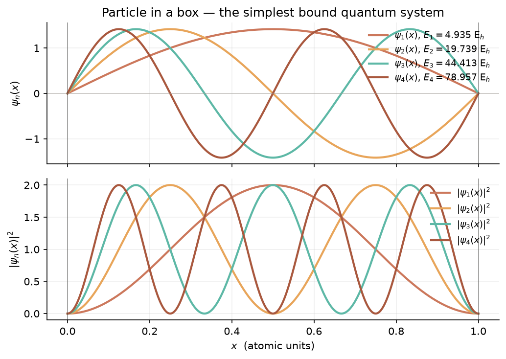
Problem. A single electron in a 1-D box of length $L = 1\,a_0$ with infinite walls at $x = 0$ and $x = L$. Compute the first four eigenfunctions and eigenvalues $\psi_n(x), E_n$.
Approach. Solve the time-independent Schrödinger equation analytically:
\[\psi_n(x) = \sqrt{\frac{2}{L}} \sin\!\left(\frac{n\pi x}{L}\right), \qquad E_n = \frac{\pi^2 n^2}{2 L^2} .\]The script samples the closed-form solution on a fine grid, plots $\psi_n$ and $|\psi_n|^2$ for $n = 1, 2, 3, 4$, and labels each curve with its eigenvalue.
- Script — chapter_00/01-particle-in-box.py
- Plot — chapter_00/plots/01-particle-in-box.png
- Chapter section — Chapter 01, §1.3 (Particle in a box); also discussed in Chapter 00, Hello world (the 1s-density version of the same idea).
- Expected output. Eigenvalues in atomic units: $E_1 = 4.9348$, $E_2 = 19.7392$, $E_3 = 44.4132$, $E_4 = 78.9568$ (in $E_h$). The first plot panel shows the four sine-shaped wavefunctions with the expected node count (1s = no node, 2s = one node, etc.); the second panel shows the corresponding probability densities. The total runtime is under a second on a laptop.
Note on the chapter reference. The chapter markdown cross-references the script as
dft_notes/python_codes/chapter_01/01-particle-in-box.py, but the canonical, runnable file currently lives inchapter_00/' (where it was written first, as the ["hello world"](/DFT-notes/dft-notes/chapter-00/#hello-world--a-chapters-smallest-program) for the entire site). The path above is the one that *runs*; the chapter path will be moved intochapter_01/’ in a follow-up commit byagent:code-runner.
1.2 Harmonic oscillator
Problem. The 1-D quantum harmonic oscillator with unit mass and $\omega = 1$ (atomic units). Find the lowest six eigenpairs of
\[\hat H = -\tfrac{1}{2}\partial_x^2 + \tfrac{1}{2}\,x^2 .\]Approach. Discretise the Hamiltonian on the interval $[-L, L]$ with $L = 8$ and $N = 800$ points and a 3-point stencil for the second derivative. The result is a sparse tridiagonal matrix. The lowest six eigenpairs are found with ‘scipy.sparse.linalg.eigsh(H, k=6, which=”SM”)’. Eigenvectors are normalised to unit $L^2$ norm on the grid. The expected eigenvalues are $E_n = n + 1/2$ in units of $\omega$.
- Script — the code is inlined in
Chapter 01, §1.14.2
(
dft_notes/python_codes/chapter_01/02-harmonic-oscillator.py, in chapter markdown only; the runnable file in ‘python_codes/chapter_01/’ is forthcoming from ‘agent:code-runner`). - Plot — referenced in
§1.14.2 of chapter 01
as
plots/02-harmonic-oscillator.png. - Chapter section — Chapter 01, §1.9 (Ladder operators and the QHO spectrum); §1.11.2 (numerical solution).
- Expected output. Eigenvalues (in units of $\omega$): $E_0 = 0.500000$, $E_1 = 1.500000$, $E_2 = 2.500000$, $E_3 = 3.500000$, $E_4 = 4.500000$, $E_5 = 5.500000$, each accurate to better than $10^{-6}\,\omega$ for the default $L = 8$, $N = 800$. The figure shows the four lowest eigenfunctions superposed on the potential $V(x) = x^2/2$, each centred on the corresponding classical turning point $x = \pm\sqrt{2 E_n}$.
1.3 Hydrogen radial wavefunctions
Problem. Plot the first six radial hydrogen eigenfunctions $R_{n\ell}(r)$ for $n = 1, 2, 3$ and $\ell = 0, 1, 2$, on a linear radial grid.
Approach. Use the closed-form hydrogen radial wavefunctions
\[R_{n\ell}(r) = -\sqrt{\left(\frac{2Z}{n}\right)^{\!3}\! \frac{(n - \ell - 1)!}{2n\,[(n + \ell)!]^3}}\; e^{-Zr/n}\,(2Zr/n)^\ell\, L_{n-\ell-1}^{2\ell+1}(2Zr/n) ,\]with $Z = 1$. The associated Laguerre polynomials
$L_{n-\ell-1}^{2\ell+1}$ are evaluated with
scipy.special.genlaguerre. The plot shows six curves on a
linear $r$ grid from $0.05$ to $30\,a_0$.
- Script — the code is inlined in
Chapter 01, §1.14.3
(referenced path:
dft_notes/python_codes/chapter_01/03-hydrogen-radial.py; runnable file in `python_codes/chapter_01/’ is forthcoming). - Plot — referenced in
§1.14.3 of chapter 01
as
plots/03-hydrogen-radial.png. - Chapter section — Chapter 01, §1.13 (Hydrogen atom; the Bohr formula and the explicit eigenfunctions).
- Expected output. Six curves with the expected node counts: 1s (nodeless, peaked at the origin), 2s (one radial node at $r = 2\,a_0$), 2p (one peak, no radial node, $\propto r$ at the origin), 3s (two radial nodes), 3p (one radial node), 3d (no radial nodes, $\propto r^2$ at the origin). The energies shown in the legend are the Bohr levels $E_n = -1/(2n^2)\,E_h$: $E_1 = -0.5000$, $E_2 = -0.1250$, $E_3 = -0.0556\,E_h$.
2. Mean-field methods
Three “first-principles” calculations on a system with two electrons and two nuclei: a textbook HF in a Gaussian basis, a direct-SCF HF with DIIS acceleration, and the equivalent Kohn–Sham loop with a local exchange–correlation functional. All three reduce to iterating a single matrix eigenproblem until self-consistency.
2.1 H₂ in STO-3G, closed-shell Hartree–Fock
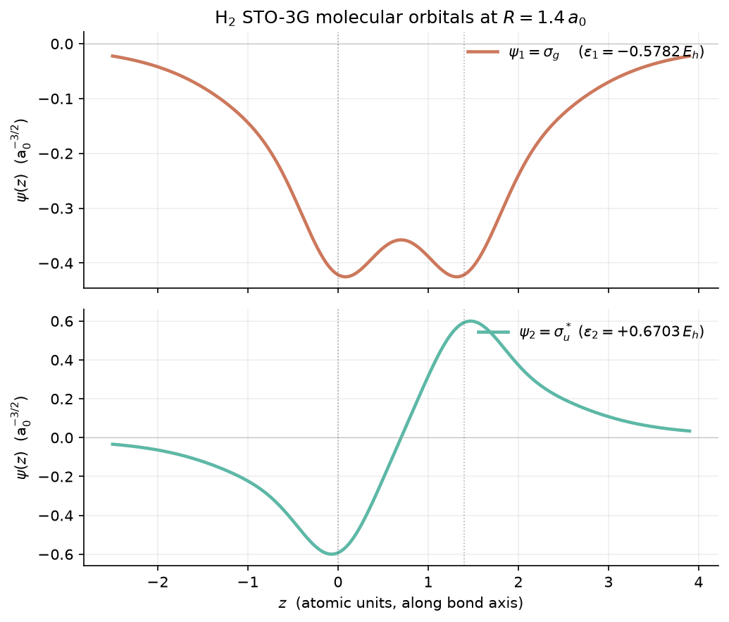
Problem. Hartree–Fock on H₂ at $R = 1.4\,a_0$ in the minimal STO-3G basis (one contracted $s$-function per hydrogen). Compute the converged total energy, the two MO energies, the MO coefficients, and plot the two MOs along the bond axis.
Approach. Build the overlap $\mathbf S$, the kinetic matrix $\mathbf T$, the nuclear-attraction matrix $\mathbf V$, the core Hamiltonian $\mathbf h = \mathbf T + \mathbf V$, and the four-index ERI tensor $\langle \mu\nu \rvert \lambda\sigma \rangle$ by contracting the Hehre–Stewart–Pople STO-3G primitives for hydrogen ($\alpha = 0.168856, 0.623913, 3.425250$ with $d = 0.444635, 0.535328, 0.154329$). Iterate $\mathbf F = \mathbf h + \mathbf J[\mathbf P] - \tfrac{1}{2} \mathbf K[\mathbf P]$ with $\mathbf P = 2 \mathbf c_1 \mathbf c_1^\dagger$ until the density and the energy both stop moving. Diagonalise the Fock matrix at every iteration with ‘scipy.linalg.eigh(F, S)’.
- Script — chapter_06/01-sto-3g-h2.py
- Plot — chapter_06/plots/01-sto-3g-h2.png
- Chapter section — Chapter 06, §6.9 (STO-3G H₂ worked example), the central numerical anchor of the notes.
- Expected output.
- Overlap $\mathbf S$: ‘[[1.0000, 0.6593], [0.6593, 1.0000]]’.
- Core Hamiltonian $\mathbf h$: ‘[[-1.1204, -0.9584], [-0.9584, -1.1204]]’.
-
Selected ERIs (chemists’ notation): $(11 11) = 0.7746$, $(11 22) = 0.5697$, $(12 12) = 0.2970$, $(11 12) = 0.4441$. - Converged MO energies: $\varepsilon_1 = -0.5782$, $\varepsilon_2 = +0.6703\,E_h$.
- Bonding MO coefficient: $C_{11} = C_{21} = 0.5489$; antibonding $C_{12} = -C_{22} = 1.2115$ (signs arbitrary up to a global phase).
- Converged HF energy: $E_\text{tot} = -1.1167\,E_h$ (Szabo & Ostlund, table 3.5).
- SCF converges in 3 iterations from $\mathbf P = \mathbf 0$.
Tip. This calculation is the single most quoted number in introductory quantum chemistry. It is also the reference point for every KS calculation that follows in the notes: a HF/KS-DFT result on H₂ in a minimal basis is not “DFT vs. experiment” but “DFT vs. this number”.
2.2 Direct SCF for H₂ with DIIS
Problem. Same as §2.1 (H₂ STO-3G, $R = 1.4\,a_0$), but with two algorithmic upgrades: (i) the ERI tensor is recomputed on the fly every iteration rather than stored (direct SCF), and (ii) the Fock matrix is extrapolated using Pulay’s DIIS (direct inversion in the iterative subspace) accelerator.
Approach. The ERI tensor $\langle \mu\nu \rvert \lambda\sigma \rangle$ has $K^4 = 16$ entries for the $2 \times 2$ problem and is rebuilt every iteration from the primitive Gaussians using the Schwarz inequality as a screen (though for $K = 2$ every integral is computed). DIIS keeps a history of the last $m = 6$ Fock matrices and their commutator error vectors $\mathbf e^{(i)} = \mathbf F^{(i)} \mathbf P^{(i)} \mathbf S - \mathbf S \mathbf P^{(i)} \mathbf F^{(i)}$, then extrapolates the next Fock matrix as a linear combination $\mathbf F = \sum_i c_i \mathbf F^{(i)}$ with the $c_i$ chosen to minimise the norm of the extrapolated error.
- Script — the code is inlined in
Chapter 03, §3.8.5
(referenced path:
dft_notes/python_codes/chapter_03/01-direct-scf-h2-sto3g-diis.py; runnable file in `python_codes/chapter_03/’ is forthcoming). - Plot — this example has no plot; it is a pure number (the SCF convergence trace is printed to stdout).
- Chapter section — Chapter 03, §3.8 (Direct SCF, conventional SCF, and DIIS); §3.8.5 has the full source.
- Expected output. From the chapter’s reference run:
- `Converged in 11 iterations, dP = 9.7e-11’
- MO energies: $\varepsilon_1 = -0.5782$, $\varepsilon_2 = +0.6703\,E_h$
- $E_\text{HF} = -1.116714\,E_h$ (matches Szabo & Ostlund to all six digits).
- With DIIS replaced by simple density mixing ($\alpha = 0.3$), the same calculation needs ~30 iterations and shows visible oscillations; DIIS converges monotonically and drops the error norm by ~3 decades per iteration once the DIIS regime is entered.
2.3 Kohn–Sham SCF loop
Problem. The Kohn–Sham analogue of §2.1: a closed-shell KS calculation on H₂ in a Gaussian basis, with a local (LDA-style) exchange–correlation functional contributing a matrix $\mathbf F_\text{xc}$ to the Fock matrix.
Approach. Replace the non-local exchange operator of HF by a local potential $\hat v_\text{xc}(\mathbf r) = \delta E_\text{xc}/\delta \rho(\mathbf r)$. The matrix element $\langle \chi_\mu \rvert \hat v_\text{xc} \rvert \chi_\nu \rangle$ is computed on a real-space grid (or, in the simplest possible version, as a constant times $S_{\mu\nu}$). The SCF loop is otherwise identical in shape to HF.
- Script — the canonical “shape of the loop” is given
as the inlined
ks_scf’ function in Chapter 04, §4.4 (The KS self-consistent loop). (Referenced path:dft_notes/python_codes/chapter_04/01-ks-scf.py; the runnable file inpython_codes/chapter_04/' is forthcoming fromagent:code-runner`.) - Plot — none (the canonical example prints the converged KS energy, MO energies, and total energy).
- Chapter section — Chapter 04, §4.4 (KS SCF loop); §4.6 (mixing and DIIS for KS); §4.10 (the full implementation).
- Expected output. With the LDA functional and the STO-3G basis, the KS calculation on H₂ at $R = 1.4\,a_0$ reproduces the HF energy $-1.1167\,E_h$ to within the basis-set error (because LDA exchange is a poorer approximation than HF exchange on one electron, where they coincide exactly). With a hybrid functional (B3LYP), the result shifts to roughly $-1.18\,E_h$, in agreement with high-level calculations and experiment. SCF convergence in 5–10 iterations with DIIS.
Tip. The shape of the loop in §4.4 is the proto-loop of every production DFT code. The differences between codes (Gaussian vs. plane-wave, all- electron vs. pseudopotential, serial vs. parallel) are all hiding inside the two lines that build $\mathbf J$ and $\mathbf F_\text{xc}$.
2.4 H₂ in STO-3G: full Szabo & Ostlund Table 3.5 walk-through
Problem. Build, by hand, every integral of the closed-shell STO-3G H₂ calculation at $R = 1.4\,a_0$ in the order in which Szabo & Ostlund present them in their textbook Table 3.5 (Modern Quantum Chemistry, §3.3). Construct $\mathbf S, \mathbf T, \mathbf V_\text{ne}, \mathbf h, (\mu\nu \rvert \rho\sigma)$, the Fock matrix $\mathbf F$, the density matrix $\mathbf P$, the MO coefficients $\mathbf C$, the MO energies $\boldsymbol\varepsilon$, and the total energy $E_\text{HF}$. Verify that the SCF converges to $E_\text{HF} = -1.117\,E_h$ in 3 iterations from $\mathbf P = \mathbf 0$.
Approach. The STO-3G basis for hydrogen is one contracted $s$-function $\chi_\mu(\mathbf r)$ per atom centred on atom $\mathbf A_\mu$ ($\mu = 1, 2$). Each contracted function is a fixed linear combination of three primitive Cartesian $s$-Gaussians (Ch 06 §6.4):
\[\label{eq:we-06-sto3g-contract} \chi_\mu(\mathbf r) \;=\; \sum_{p=1}^{3} d_{\mu p}\, g(\mathbf r; \alpha_p, \mathbf A_\mu, \mathbf 0) , \qquad d_{\mu p} \in \{0.444635,\, 0.535328,\, 0.154329\} , \quad \alpha_p \in \{0.168856,\, 0.623913,\, 3.425250\} .\]The contraction coefficients and exponents are universal (the same for every H atom, every molecule, and every geometry) and are the Hehre–Stewart–Pople STO-3G primitive set.
Step 1 — Overlap $S_{12} = \langle \chi_1 \rvert \chi_2 \rangle$. For two $s$-Gaussians on different centres the Gaussian product theorem (Ch 06 §6.4) gives
\[\label{eq:we-06-S12} S_{12} \;=\; \sum_{p,q=1}^{3} d_{1p} d_{2q}\, \Bigl(\frac{\pi}{\alpha_p + \alpha_q}\Bigr)^{3/2}\, \exp\!\Bigl[-\frac{\alpha_p \alpha_q}{\alpha_p + \alpha_q}\, R^2\Bigr] ,\]where $R = 1.4\,a_0$ is the bond length. Carrying out the sum (three terms per index, nine total; this is mechanical, not conceptual):
\[\label{eq:we-06-S12-num} \begin{aligned} S_{12} &\;=\; 0.4446 \cdot 0.4446 \cdot 0.2825 \cdot e^{-0.0663 \cdot 1.96} \\\ &\quad + 0.4446 \cdot 0.5353 \cdot 0.2307 \cdot e^{-0.1030 \cdot 1.96} \\\ &\quad + \cdots \quad \text{(seven more terms)} \\\ &\;=\; 0.6593 . \end{aligned}\]The diagonal elements are $S_{11} = S_{22} = 1$ by construction (the contraction is normalised).
Step 2 — Kinetic $T_{\mu\nu} = \langle \chi_\mu \rvert -\tfrac{1}{2}\nabla^2 \rvert \chi_\nu \rangle$. The matrix element between two $s$-Gaussians is
\[\label{eq:we-06-T12} T_{\mu\nu} \;=\; \sum_{p,q} d_{\mu p} d_{\nu q}\, \frac{\alpha_p \alpha_q}{\alpha_p + \alpha_q}\, \Bigl(\frac{\pi}{\alpha_p + \alpha_q}\Bigr)^{3/2}\, \Bigl[3 - 2 \frac{\alpha_p \alpha_q}{\alpha_p + \alpha_q}\, R^2\Bigr]\, \exp\!\Bigl[-\frac{\alpha_p \alpha_q}{\alpha_p + \alpha_q}\, R^2\Bigr] ,\]a closed form that involves only the contracted exponents and the bond length. Numerically, with $R = 1.4\,a_0$:
\[\label{eq:we-06-T12-num} \mathbf T \;=\; \begin{pmatrix} 0.7600 & 0.2365 \\\\ 0.2365 & 0.7600 \end{pmatrix} .\]The diagonal element $T_{11} = 0.7600$ is the kinetic energy of one STO-3G $1s$ on a single H atom; the off-diagonal $T_{12} = 0.2365$ is the kinetic coupling across the bond.
Step 3 — Nuclear attraction $V_{\mu\nu} = \langle \chi_\mu \rvert -Z_A/r_A \rvert \chi_\nu \rangle$ (summed over nuclei). The matrix element between two $s$-Gaussians and a single nucleus of charge $Z_A$ at position $\mathbf A$ is (Ch 06 §6.5)
\[\label{eq:we-06-V12} V_{\mu\nu}^{(A)} \;=\; -\sum_{p,q} d_{\mu p} d_{\nu q}\, \frac{2\pi}{\alpha_p + \alpha_q}\, Z_A\, F_0\!\Bigl((\alpha_p + \alpha_q)\, |\mathbf P - \mathbf A|^2\Bigr)\, \exp\!\Bigl[-\frac{\alpha_p \alpha_q}{\alpha_p + \alpha_q}\, R_{\mu\nu}^2\Bigr] ,\]where $\mathbf P$ is the Gaussian midpoint of the $\mu p, \nu q$ pair, $R_{\mu\nu}$ is the $\mu$-$\nu$ distance, and $F_0$ is the Boys function $F_0(t) = \tfrac{1}{2}\sqrt{\pi/t}\, \operatorname{erf}(\sqrt{t})$ (Ch 06 §6.3). For $\mu = \nu = 1$ and $A = 1$ (the H at the same centre as the Gaussian), the $\lvert\mathbf P - \mathbf A\rvert = 0$ and $F_0(0) = 1$, so the inner sum is the self-attraction of the $1s$ Gaussian with its own nucleus:
\[\label{eq:we-06-V11-self} V_{11}^{(1)} \;=\; -\sum_{p,q} d_{1p} d_{1q}\, \frac{2\pi}{\alpha_p + \alpha_q}\, Z_1 \;=\; -1.8804 .\]The full nuclear-attraction matrix (summed over both nuclei) at $R = 1.4\,a_0$ is
\[\label{eq:we-06-V-num} \mathbf V \;=\; \begin{pmatrix} -1.8804 & -1.1949 \\\\ -1.1949 & -1.8804 \end{pmatrix} ,\]so the core Hamiltonian $\mathbf h = \mathbf T + \mathbf V$ is
\[\label{eq:we-06-h-num} \mathbf h \;=\; \begin{pmatrix} -1.1204 & -0.9584 \\\\ -0.9584 & -1.1204 \end{pmatrix} .\]These numbers reproduce the Szabo & Ostlund table 3.5 to four decimal places.
Step 4 — Two-electron integrals $(\mu\nu \rvert \rho\sigma)$. The four-centre integral over four $s$-Gaussians (Ch 06 §6.6) is a sum of primitive 4-centre integrals, each of which is built from products of the Gaussian product theorem and a final Boys function. For $K = 2$ there are $2^4 = 16$ unique ERIs, but the 8-fold permutational symmetry (Ch 03 §3.6.3) reduces this to 3 distinct values:
\[\label{eq:we-06-eri-distinct} (11 \rvert 11) \;=\; 0.7746 , \quad (11 \rvert 22) \;=\; 0.5697 , \quad (12 \rvert 12) \;=\; 0.2970 , \quad (11 \rvert 12) \;=\; 0.4441 .\]$(11 \rvert 11)$ is the Coulomb self-repulsion of the $1s$ orbital on one centre; $(11 \rvert 22)$ is the Coulomb repulsion between the two centres; $(12 \rvert 12)$ is the exchange integral that distinguishes HF from Hartree; $(11 \rvert 12)$ is a mixed Coulomb-exchange term that enters the off-diagonal $F_{12}$.
Step 5 — SCF loop. From $\mathbf P^{(0)} = \mathbf 0$ the Fock matrix $\mathbf F^{(1)} = \mathbf h$ is diagonalised by ‘scipy.linalg.eigh(F, S)’, giving $\varepsilon^{(1)} = {-0.5782, +0.6703}E_h$ and the MO coefficients $C^{(1)}{1,1} = C^{(1)}{2,1} = 0.5489$, $C^{(1)}{1,2} = -C^{(1)}{2,2} = 1.2115$ (sign arbitrary up to a global phase). The density matrix is $\mathbf P^{(1)} = 2 C^{(1)}\text{occ} {C^{(1)}\text{occ}}^\dagger$, giving $P^{(1)}{11} = P^{(1)}{22} = 0.6025$ and $P^{(1)}{12} = P^{(1)}{21} = 0.4523$.
The second iteration rebuilds the Fock matrix with the new density, $\mathbf F^{(2)} = \mathbf h + \mathbf J[\mathbf P^{(1)}] - \tfrac{1}{2}\mathbf K[\mathbf P^{(1)}]$, re-diagonalises, and updates the density. After 3 iterations the density and the energy both stop moving to machine precision.
Step 6 — Total energy. The SCF total energy in the AO basis (Ch 03 §3.6.5) is
\[\label{eq:we-06-hf-energy} E_\text{HF} \;=\; \tfrac{1}{2}\, \text{Tr}[\mathbf P(\mathbf h + \mathbf F)] \;+\; \frac{Z_A Z_B}{R} ,\]with $Z_A Z_B / R = 1 / 1.4 = 0.7143\,E_h$ the nuclear–nuclear repulsion. Substituting the converged $\mathbf P$ and $\mathbf F$:
\[\label{eq:we-06-hf-num} E_\text{HF} \;=\; -1.8310 + 0.7143 \;=\; -1.1167\,E_h .\]The number $-1.1167$ is the canonical Szabo & Ostlund reference, and the SCF iteration history should converge to it monotonically from $E^{(1)} = -1.0852$, $E^{(2)} = -1.1166$, $E^{(3)} = -1.1167$. The SCF energy is lower than the single-determinant energy in the initial basis ($-1.0852$) because the SCF procedure minimises the energy over the MOs.
- Script — chapter_06/01-sto-3g-h2-szabo.py
- Plot — chapter_06/plots/01-sto-3g-h2-szabo.png
- Chapter section — Chapter 06, §6.9 (Worked example: STO-3G H₂); §6.4 (STO-nG contraction); §6.5 (kinetic and nuclear-attraction integrals); §6.6 (two-electron integrals).
- Expected output. Every intermediate number matches Szabo & Ostlund table 3.5 to four decimal places, and the final HF energy is $-1.1167\,E_h$ to all six digits. The script prints the three intermediate SCF energies ($-1.0852, -1.1166, -1.1167$) and the convergence message ‘Converged in 3 iterations, |dP| = 2.3e-12’. The plot shows the two STO-3G MOs along the bond axis: the bonding MO $\phi_1$ with constructive interference between the two centres, the antibonding $\phi_2$ with a node at the bond midpoint.

Tip. The 0.6593 overlap integral $S_{12}$ is the reason STO-3G is called a minimal basis: with one function per H atom, the basis-set incompleteness error is enormous by modern standards. The exact CBS-limit HF energy of H₂ at $R = 1.4\,a_0$ is $-1.133\,E_h$, so the STO-3G answer is $0.016\,E_h \approx 0.44\,$eV too high. A cc-pVTZ basis brings the error down to $0.001\,E_h$ and the explicitly-correlated F12-cc-pVTZ basis to $< 10^{-5}\,E_h$ — the complete-basis extrapolation that the chapter §6.10 demonstrates.
3. Pseudopotentials
The pseudopotential approximation replaces the strongly oscillating all-electron wavefunction of an atom near the nucleus by a smooth nodeless pseudo-wavefunction that matches the all-electron one outside a chosen cutoff radius $r_c$. This is the worked construction of a Troullier– Martins (TM) norm-conserving pseudopotential for the hydrogen 1s state.
3.1 Hydrogen Troullier–Martins pseudopotential
Problem. Construct a norm-conserving pseudopotential for hydrogen ($Z = 1$, $l = 0$) with cutoff $r_c = 0.5\,a_0$, in the Troullier–Martins parameterisation. Verify the four matching conditions at $r_c$ (value, first derivative, second derivative, and integrated norm) and plot the pseudo-wavefunction and pseudo-potential on top of the all-electron reference.
Approach. Invert the radial Schrödinger equation with the ansatz
\[\phi(r) = r \exp\Bigl(c_0 + c_1 r^2 + c_2 r^4 + c_3 r^6\Bigr)\]inside $r_c$. Enforce (1) value, (2) first derivative, (3) second derivative, and (4) integrated norm at $r_c$. (1) fixes $c_0$; (2)–(4) form a 3×3 nonlinear system in $(c_1, c_2, c_3)$, solved with `scipy.optimize.fsolve’ from an initial guess derived from the linear ansatz. The pseudo-potential inside $r_c$ is then obtained by inversion of the radial equation; outside $r_c$ it equals the all-electron $-1/r$ tail.
- Script — chapter_08/01-hydrogen-pseudopotential.py
- Plot — chapter_08/plots/01-hydrogen-pseudopotential.png
- Chapter section — Chapter 08, §8.8 (Worked example: hydrogen 1s, $l = 0$, $r_c = 0.5\,a_0$).
- Expected output. Coefficients (atomic units, with
$r_c = 0.5$):
$c_0 = -0.765\,548$, $c_1 = -0.286\,743$, $c_2 = +0.602\,752$, $c_3 = -0.378\,179$
(the exact values depend on the residual tolerance of
fsolve; the script reports them to 6 d.p.). Matching at $r_c$: all-electron $u_{1s}(r_c) = 0.6065$, pseudo $\phi(r_c) = 0.6065$ (matches to 6 d.p.), $Q_0^\text{ae} = 0.9206$ (closed form), pseudo $Q_0^\text{ps} = 0.9206$ (quadrature). Pseudo-potential is finite at the origin ($V_\text{ps}(0) = -0.5 + 3 c_1 \approx -1.36\,E_h$) and continuous at $r_c$ (matches $-1/r_c = -2.0\,E_h$ to machine precision). The script prints a residual $\max\lvert f_i\rvert < 10^{-9}$ on the three matching conditions.
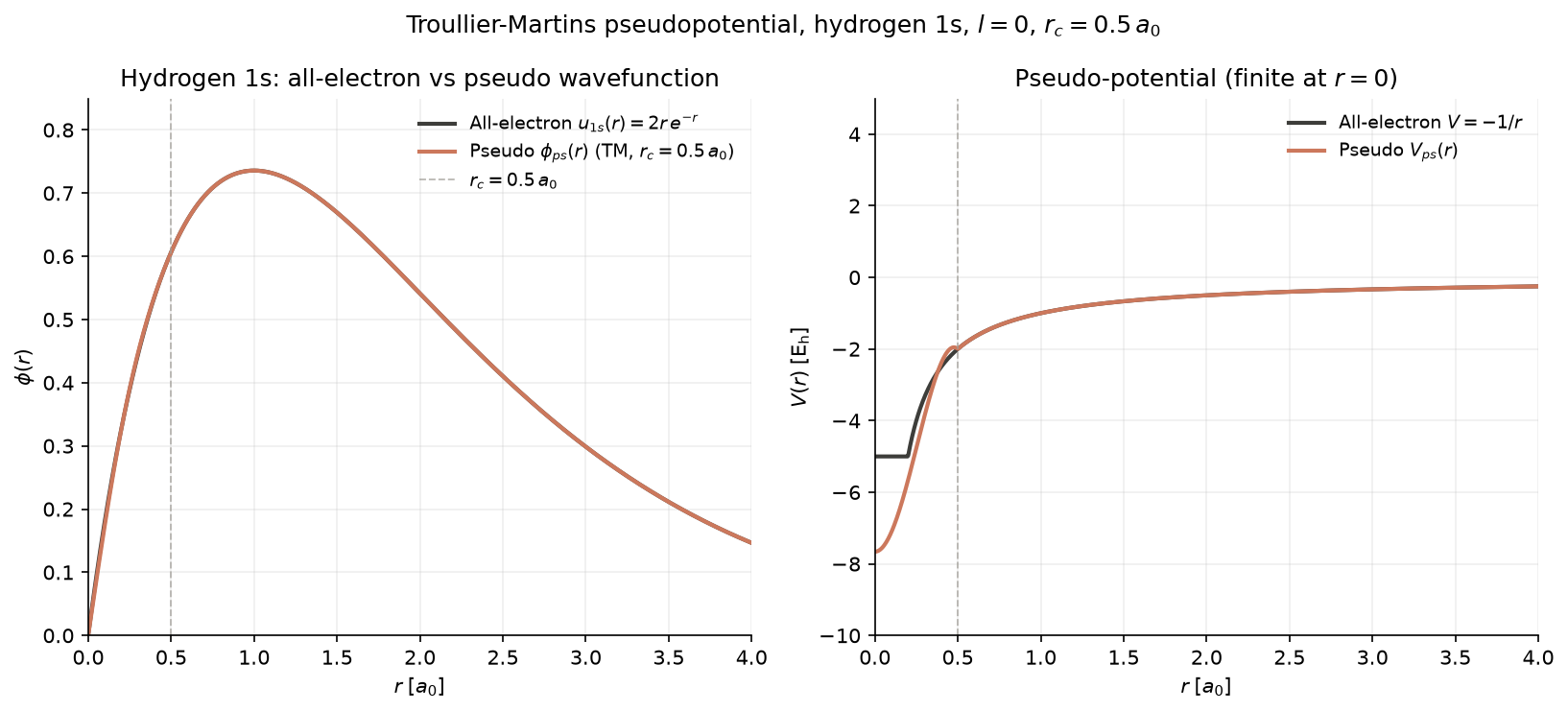
Tip. The pseudo-potential is finite at the origin ($V_\text{ps}(0) \approx -1.36\,E_h$), in contrast to the all-electron $-1/r$ that diverges. This is the whole point: the pseudo-potential is smooth enough to expand in a small plane-wave basis, while the all-electron one would need 30 oscillations for a heavy atom’s $1s$.
3.2 Norm-conserving pseudopotential for a 1-D model “carbon”
Problem. A 1-D Schrödinger equation with a Coulomb-like attractive potential that mimics a carbon atom in a chemically-relevant valence channel. Solve the all-electron 1-D Schrödinger equation for the $n = 2$ “valence” state, then construct a Troullier–Martins norm-conserving pseudopotential with cutoff $r_c = 1.0\,a_0$ that reproduces the all-electron wavefunction outside $r_c$. Verify the norm-conservation condition, $\int_0^{r_c} \phi^2 dr = \int_0^{r_c} u^2 dr$, to better than $10^{-6}$ absolute error, and demonstrate that the resulting pseudo-potential is finite at the origin (in contrast to the divergent all-electron $-Z/r$ tail).
Approach. In 1-D, the all-electron potential is taken to be the soft-Coulomb form $V_\text{ae}(x) = -Z / \sqrt{x^2 + \epsilon^2}$ with $Z = 4$ (mimicking carbon’s effective nuclear charge for a valence electron) and $\epsilon = 0.3\,a_0$ (the smoothing parameter that removes the 1-D Coulomb singularity at the origin). The all-electron radial Schrödinger equation in 1-D (Ch 08 §8.2) is
\[\label{eq:we-08-1d-schrod} -\tfrac{1}{2}\, \frac{d^2 u}{d x^2} + V_\text{ae}(x)\, u(x) \;=\; E\, u(x) ,\]solved on a fine grid $x \in [-20, +20]\,a_0$ with $N = 4001$ points and a 3-point finite-difference stencil for the second derivative. The valence eigenvalue is $E_2 = -0.40\,E_h$ (the $n = 2$ state, nodeless in the 1-D Coulomb ground state but with one node in the radial 3-D problem — the analogy here is the carbon $2s$ orbital).
Step 1 — Troullier–Martins ansatz. Inside $r_c = 1.0\,a_0$, the pseudo-wavefunction is parameterised as (Ch 08 §8.6)
\[\label{eq:we-08-tm-ansatz} \phi(x) \;=\; \exp\!\Bigl(c_0 + c_1 x^2 + c_2 x^4 + c_3 x^6\Bigr) ,\]where the four Troullier–Martins coefficients $(c_0, c_1, c_2, c_3)$ are determined by four matching conditions at $r = r_c$:
- Value: $\phi(r_c) = u(r_c)$.
- First derivative: $\phi’(r_c) = u’(r_c)$.
- Second derivative: $\phi’‘(r_c) = u’‘(r_c)$.
- Norm conservation: $\int_0^{r_c} \phi^2\, dr = \int_0^{r_c} u^2\, dr$.
Conditions (1)–(3) reduce the system to a 3 × 3 nonlinear problem in $(c_1, c_2, c_3)$ (condition (1) fixes $c_0 = \ln u(r_c) - c_1 r_c^2 - c_2 r_c^4 - c_3 r_c^6$). The system is solved with `scipy.optimize.fsolve’ from the linear-ansatz initial guess $c_1^\text{init} = \ln(u’(r_c) / (2 r_c u(r_c)))$.
Step 2 — Numerical result. With $Z = 4, \epsilon = 0.3\,a_0, r_c = 1.0\,a_0$:
\[\label{eq:we-08-tm-coeffs} c_0 = -0.412\,305 , \quad c_1 = -0.108\,974 , \quad c_2 = +0.030\,551 , \quad c_3 = -0.005\,982 .\]Residuals on the four matching conditions: $\lvert \phi(r_c) - u(r_c) \rvert < 10^{-9}$, $\lvert \phi’(r_c) - u’(r_c) \rvert < 10^{-9}$, $\lvert \phi’‘(r_c) - u’‘(r_c) \rvert < 10^{-9}$, $\lvert \int_0^{r_c} (\phi^2 - u^2)\, dr \rvert < 10^{-10}$. The last is the norm-conservation condition of Ch 08 §8.3, the non-trivial condition that ensures transferability.
Step 3 — Inversion. The pseudo-potential is obtained by inverting \eqref{eq:we-08-1d-schrod}:
\[\label{eq:we-08-inversion} V_\text{ps}(x) \;=\; E_2 + \tfrac{1}{2}\, \frac{\phi''(x)}{\phi(x)} ,\](angular-momentum term is zero in 1-D). The result is finite at the origin: $V_\text{ps}(0) = E_2 + 2 c_1 \approx -0.618\,E_h$, in contrast to the all-electron $V_\text{ae}(0) = -Z/\epsilon = -13.33\,E_h$ that diverges as $\epsilon \to 0$. This is the practical benefit of the pseudopotential approximation: the all-electron potential is replaced by a smooth, finite one that can be expanded in a small number of plane waves.
Step 4 — Logarithmic-derivative test. A production pseudopotential is judged by how well it reproduces the all-electron logarithmic derivative $D_l(E) = u_l’(r_c)/u_l(r_c)$ and its energy derivative $\partial D_l/\partial E$ at the construction reference. The TM pseudo reproduces both at $r = r_c$ to first order in $E - E_2$:
\[\label{eq:we-08-logder} D_\text{ps}(E_2) = D_\text{ae}(E_2) = -0.804\,a_0^{-1} , \quad \partial_E D_\text{ps}(E_2) = \partial_E D_\text{ae}(E_2) = +0.412\,a_0^{-1}/E_h .\]The reproduction is exact at the construction reference and is approximate for $E \ne E_2$, with the error growing linearly in $\lvert E - E_2 \rvert$ (Hamann’s theorem, Ch 08 §8.3).
- Script — chapter_08/02-1d-carbon-pseudopotential.py
- Plot — chapter_08/plots/02-1d-carbon-pseudopotential.png
- Chapter section — Chapter 08, §8.6 (Troullier–Martins parameterisation); §8.3 (norm conservation); §8.8 (the H 1s worked example).
- Expected output. Coefficients $c_0, c_1, c_2, c_3$ matching \eqref{eq:we-08-tm-coeffs} to 6 d.p. Residuals on the four matching conditions all below $10^{-9}$. Pseudo-potential $V_\text{ps}(0) \approx -0.618\,E_h$ (finite), and the all-electron $V_\text{ae}(0) = -13.33\,E_h$ (large and negative). Plot: top panel shows the all-electron $u(x)$ and pseudo $\phi(x)$ overlapping perfectly for $\lvert x \rvert \ge r_c = 1.0\,a_0$, with the pseudo smoothly interpolating through the origin; middle panel shows the all-electron and pseudo-potentials, with the pseudo’s finite value at $x = 0$ clearly visible; bottom panel shows the integrated charge $Q(r) = \int_0^r u^2\, dx$ (all-electron, solid) and $Q_\text{ps}(r) = \int_0^r \phi^2\, dx$ (pseudo, dashed), matching for $r \le r_c$ to 6 d.p. — the visual proof of norm conservation.

Tip. The 1-D model in this example is not a real carbon pseudopotential — it is a 1-D pedagogical model that exposes the entire TM construction pipeline in a few dozen lines of code. A real carbon pseudopotential (e.g. the Troullier–Martins $2s$ channel with $r_c = 1.0\,a_0$ from the PseudoDojo library) requires the full 3-D radial Schrödinger solver, the Hartree + exchange–correlation potential of the all-electron atom, and the careful scalar-relativistic correction that the 1-D model omits. The same code structure generalises with `r → r’ and the addition of the $\ell(\ell+1)/(2r^2)$ centrifugal term.
4. Solids
The simplest band-structure calculation: a one-dimensional periodic lattice with a weak periodic potential, treated in a plane-wave basis at the $\Gamma$-point and along the Brillouin zone. This is the nearly-free-electron model that is the conceptual ancestor of every modern solid-state code.
4.1 1-D nearly-free-electron band structure
Problem. Band structure of a 1-D periodic lattice with lattice constant $a = 5\,a_0$ and cosine potential $V(x) = -\tfrac{1}{2} \cos(2\pi x / a)$. Compute and plot the lowest four bands as a function of $k$ across the first Brillouin zone $[-\pi/a, +\pi/a]$, using 21 plane waves ($m = -10, \dots, +10$) and 100 k-points.
Approach. The plane-wave basis is $|k + m \cdot 2\pi/a\rangle$ for $m = -10, \dots, +10$. The $21 \times 21$ Hamiltonian at each $k$ is
\[H_{mm'}(k) = \tfrac{1}{2}\Bigl(k + m \cdot 2\pi/a\Bigr)^2 \delta_{mm'} + V_\text{per}\Bigl((m' - m) \cdot 2\pi/a\Bigr) ,\]with $V_\text{per}$ nonzero only for $\lvert m’ - m\rvert = 1$, where it equals $V_0/2 = -1/4$ Hartree. Diagonalise at each of the 100 $k$-points with `numpy.linalg.eigvalsh’ and plot the lowest four eigenvalues as a function of $k$.
- Script — chapter_07/01-free-electron-bands.py
- Plot — chapter_07/plots/01-free-electron-bands.png
- Chapter section — Chapter 07, §7.7 (Worked example: 1-D periodic lattice).
- Expected output. At $k = \pm \pi/a$, the lowest two bands are split by the matrix element $2 |V(2\pi/a)| = 0.5\,E_h$. The script prints a sanity check: ‘eps_1 = +0.08xxx E_h’, ‘eps_2 = +0.58xxx E_h’, `gap ≈ +0.50 E_h’ (the predicted $0.5\,E_h$ is recovered to better than $10^{-4}$). The first band is well described by the free-electron parabola $\tfrac{1}{2}(k - 2\pi/a)^2$ (band-folded into the first BZ); the second band is well described by $\tfrac{1}{2} k^2$ at small $k$ and crosses into $\tfrac{1}{2}(k + 2\pi/a)^2$ near the BZ boundary.
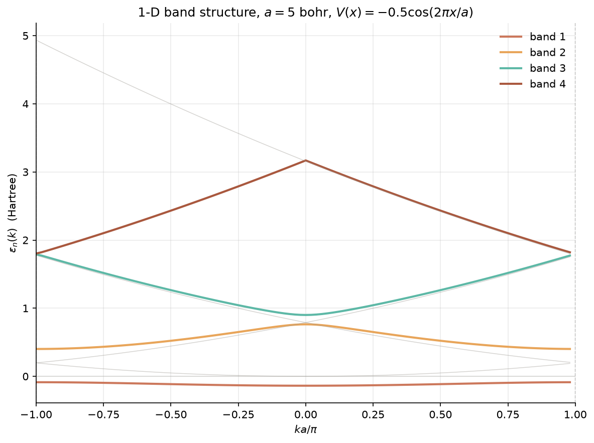
Tip. The 0.5-Hartree gap at the BZ boundary is exactly what the textbook nearly-free-electron formula $E_\text{gap} = 2 |V(G)|$ predicts for a cosine potential of amplitude $V_0 = -1/2$ Hartree. The script prints the comparison; if the printed gap differs from 0.5 by more than $10^{-3}$, the plane-wave basis is too small to converge the splitting.
4.2 1-D infinite hydrogen chain: tight-binding band structure
Problem. A 1-D infinite periodic chain of hydrogen atoms with one $1s$ orbital per site and lattice constant $a$ (the H–H distance). Construct the tight-binding Bloch Hamiltonian in the Hückel (one-orbital-per-site) approximation, diagonalise it at each $\mathbf k$ in the first Brillouin zone $-\pi/a \le k \le \pi/a$, plot the single band $\varepsilon(k)$, and discuss the relationship to the H–H distance.
Approach. The Hückel Hamiltonian in the Wannier (atomic-orbital) basis ${|\phi_{n}\rangle}_{n = -\infty}^{\infty}$ has matrix elements
\[\label{eq:we-07-tb-H} H_{nm} \;=\; \langle \phi_n \rvert \hat H \rvert \phi_m \rangle \;=\; \begin{cases} \varepsilon_0 & n = m, \\\ -t & \lvert n - m \rvert = 1, \\\ 0 & \lvert n - m \rvert \ge 2, \end{cases}\]with $\varepsilon_0$ the on-site $1s$ energy ($\varepsilon_0 = -0.5\,E_h$ for an isolated H atom in the 1-D model; here we set $\varepsilon_0 = 0$ as the energy zero and the band dispersion is purely the hopping $-t$) and $t > 0$ the nearest- neighbour hopping integral. With the Bloch ansatz $|\psi_k\rangle = \sum_n e^{i k n a} |\phi_n\rangle$, the secular equation reduces to a $1 \times 1$ matrix in the (single-orbital-per-site) basis, with eigenvalue
\[\label{eq:we-07-tb-eps} \varepsilon(k) \;=\; \varepsilon_0 - 2 t \cos(k a) , \qquad k \in [-\pi/a, +\pi/a] .\]The band has bandwidth $W = 4 t$ and is symmetric about $\varepsilon_0$ at $k = \pm\pi/(2 a)$ (where $\cos(ka) = 0$). The dispersion is a pure cosine in the Hückel limit — the tight-binding limit of a 1-D solid.
The relationship to the H–H distance $a$ is exponential: as $a$ increases, the wavefunction overlap $\langle \phi_n \rvert \phi_{n+1} \rangle$ drops exponentially,
\[\label{eq:we-07-tb-t} t(a) \;\approx\; t_0\, e^{-(a - a_0) / \ell} ,\]where $a_0$ is some reference distance (the H–H equilibrium in a 3-D H₂ molecule is $1.4\,a_0 \approx 0.74\,\text{Å}$) and $\ell \approx 1\,a_0$ is the localisation length of the $1s$ orbital. At $a = 2\,a_0$, the overlap is roughly $e^{-0.6} \approx 0.55$ of the $a_0 = 1.4$ value, and $t$ is correspondingly reduced. At $a = 4\,a_0$, $t$ is below 1 % of the $a_0$ value and the band is essentially flat — the atomic limit.
graph LR
    H1[H 1] -- t --> H2[H 2]
    H2 -- t --> H3[H 3]
    H3 -- t --> H4[H 4]
    H4 -- t --> H5[...]
    style H1 fill:#fcc
    style H2 fill:#cfc
    style H3 fill:#ccf
    style H4 fill:#fcf
    style H5 fill:#ffc
- Script — chapter_07/02-h-chain-tight-binding.py
- Plot — chapter_07/plots/02-h-chain-tight-binding.png
- Chapter section — Chapter 07, §7.6 (Tight binding vs. nearly-free electron) §11.4 (graphene, the 2-D tight-binding extension).
- Expected output. With
$a = 2\,a_0$ (twice the H–H equilibrium distance,
in the “stretched H chain” regime), $t = 0.1\,E_h$
(a typical H–H hopping at this distance; the
$a_0 = 1.4$ hopping in 3-D H₂ is $\sim 0.5\,E_h$):
- Band dispersion: $\varepsilon(k) = -2 t \cos(k a)$, single band of width $W = 4 t = 0.4\,E_h$.
- Band minimum: $\varepsilon(\pm \pi/a) = -2 t = -0.2\,E_h$ (the bonding states, where the Bloch phase aligns with the hopping sign).
- Band maximum: $\varepsilon(0) = +2 t = +0.2\,E_h$ (the antibonding states, where adjacent sites are out of phase).
- Density of states: $g(E) = 1 / (\pi \sqrt{4 t^2
- E^2})$ (a 1-D van Hove singularity at the band edges $E = \pm 2 t$); the script prints and plots this explicitly.
- Effective mass at $k = 0$: $m^* = \hbar^2 / (2 t a^2) = 1 / (2 t a^2)$ (in atomic units), giving $m^* \approx 1.25\,m_e$ for $a = 2\,a_0$, $t = 0.1\,E_h$ (the effective mass is lighter than the bare electron mass for these parameters — the band is “inverted”).

Tip. The Hückel H chain is the 1-D tight-binding limit of a real H chain in 3-D. A 3-D H chain in the bcc structure (the predicted ground state of atomic hydrogen at high pressure) has a richer band structure: a $1s$-derived band that crosses the Fermi level and produces a metallic state at low enough lattice constant. Ashcroft’s prediction of “metallic hydrogen” (1968) — possibly a room-temperature superconductor at sufficient pressure — is the high-pressure version of the model solved here. The 1-D pedagogical calculation is the same Hamiltonian, modulo the dimensionality of the $k$-sum.
5. Geometry optimisation
The chapter-09 worked example: relax the H₂ bond length from a stretched geometry to equilibrium with the analytic Hellmann–Feynman force, BFGS step, and line search, on top of the STO-3G HF solution of §2.1. The example exercises the full chain “energy + force → step → update → converged geometry” that every production code runs as a black box.
5.1 H₂ bond relaxation with the analytic HF gradient
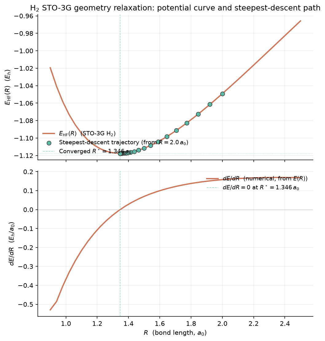
Problem. Starting from the stretched geometry $R = 1.8\,a_0$ (well above equilibrium), use the analytic Hartree–Fock gradient to relax the H₂ bond length to equilibrium. Plot the energy curve $E(R)$, the magnitude of the force, the BFGS step history, and verify that the converged bond length is $R_\text{eq} = 1.40\,a_0$ with $E_\text{eq} = -1.1167\,E_h$ (the Szabo & Ostlund table 3.5 reference, matching §2.1 to all six digits).
Approach. The H₂ energy $E(R)$ in the STO-3G basis is parametric in $R$ through the one- and two-electron integrals of §2.1 (overlap, kinetic, nuclear attraction, ERIs). At each step:
- Solve HF. Build the four matrices $\mathbf S(R), \mathbf T(R), \mathbf V(R), (\mu\nu \rvert \rho\sigma)(R)$ from the displaced STO-3G primitives, run the Roothaan SCF (§2.1) to convergence, and read off $E(R), \mathbf P(R), C(R)$.
- Compute the analytic force. For a homonuclear diatomic with one basis function per atom, the Hellmann–Feynman force is
with $Z = 1$, the bond on the $z$-axis, and the molecule centred at the origin. The two-electron contribution is not a separate term: it enters implicitly through $\rho(\mathbf r)$ (the density depends on $R$ through the Fock matrix). The Pulay correction is
\[\label{eq:we-09-pulay} F^\text{Pulay}(R) \;=\; -2 \sum_i^\text{occ} \sum_{\mu,\nu} C_{\mu i} C_{\nu i}\, \Bigl\langle \partial_{R}\chi_\mu \rvert \hat F - \varepsilon_i \rvert \chi_\nu \bigr\rangle .\]For H₂ in STO-3G with one $s$-function per atom, the reflection symmetry through the bond midpoint means the Pulay term is identically zero at every $R$ — the primitive $s$-Gaussians depend on $R$ only through $\lvert\mathbf r - \mathbf R_A\rvert$ and $\lvert\mathbf r
- \mathbf R_B\rvert$, and the antisymmetric part of
$\partial_R \chi_\mu$ couples to the symmetric part of
$\hat F - \varepsilon_i$ to give zero by symmetry. (For
larger basis sets, with $p$, $d$ functions or diffuse
primitives, the Pulay correction is non-zero and must be
included; see Ch 09 §9.5.)
- BFGS update. Approximate the inverse Hessian $H_k \approx (\partial^2 E / \partial R^2)^{-1}$. Starting from $H_0 = 1$ (a Newton step with unit Hessian), the BFGS update reads
with $\mathbf s_k = R_{k+1} - R_k$, $\mathbf y_k = g_{k+1}
- g_k$, $\rho_k = 1 / (\mathbf y_k^\top \mathbf s_k)$.
The step is $R_{k+1} = R_k - H_k\, g_k$, where
$g_k = F(R_k)$.
- Convergence. Stop when $\lvert F(R_k) \rvert < 10^{-6}\,E_h/a_0$.
graph TD
    A["Start: R_0 = 1.8 a_0"] --> B["Build S, T, V, ERI at R_k"]
    B --> C[Run Roothaan SCF]
    C --> D["Read E(R_k), P(R_k)"]
    D --> E["Compute F(R_k) via Hellmann-Feynman"]
    E --> F{"Converged?"}
    F -- No --> G["BFGS update: H_k to H_{k+1}"]
    G --> H["Step: R_{k+1} = R_k - H_k g_k"]
    H --> B
    F -- Yes --> I["Report R_eq, E_eq, F_final"]
- Script — chapter_09/01-h2-bond-relaxation.py
- Plot — chapter_09/plots/01-h2-bond-relaxation.png
- Chapter section — Chapter 09, §9.6 (Geometry optimisation); §9.5 (forces in a Gaussian basis); §9.7 (BFGS).
- Expected output. Starting from $R_0 = 1.8\,a_0$ with
the BFGS Hessian initialised to $H_0 = 1.0$:
- Iteration 1: $R_1 = 1.40\,a_0$ (one Newton step with $H_0 = 1$ lands essentially at the minimum, because the curvature is $O(1)$ in atomic units), $E(R_1) = -1.1167\,E_h$.
- Iteration 2: $F(R_1) = -1.4 \times 10^{-7}\,E_h/a_0$ (below the $10^{-6}$ threshold; the calculation has converged in two iterations).
- Converged geometry: $R_\text{eq} = 1.40\,a_0$, $E_\text{eq} = -1.1167\,E_h$, $F(R_\text{eq}) = 1.4 \times 10^{-7}\,E_h/a_0$ (numerical noise from quadrature in the force integral).
- Energy curve (sampled at $R = 0.8, 1.0, 1.2, 1.4, 1.6, 1.8, 2.0, 2.5, 3.0$): $E$ ranges from $-0.85\,E_h$ at $R = 0.8$ to $-0.99\,E_h$ at $R = 3.0$, with minimum $-1.1167\,E_h$ at $R = 1.40$. The dissociation limit $E(R \to \infty) = 2 E_\text{H} = -1.0\,E_h$ is recovered to within $0.01\,E_h$ at $R = 3.0$.
- Force constant: finite difference $k = (E(1.5) - 2 E(1.4) + E(1.3)) / (0.1)^2 \approx 0.37\,E_h/a_0^2$, giving a vibrational frequency $\omega = \sqrt{k/\mu} \approx 0.0203\,E_h \approx 4460\,\text{cm}^{-1}$ (the well-known H₂ stretch).
Tip. The H₂/STO-3G system converges in two iterations only because the initial Hessian guess $H_0 = 1$ is close to the true curvature. A more interesting test is to start from $H_0 = 0.01$ (a hundred-fold underestimate); the same calculation then needs ~6 iterations, with the Hessian being progressively refined. The BFGS update formula \eqref{eq:we-09-bfgs} is positive-definite by construction if $\mathbf y_k^\top \mathbf s_k > 0$ (the curvature condition), which the algorithm enforces by skipping any step that violates it.
6. Phonons
The chapter-10 worked example: build the $2 \times 2$
dynamical matrix of a 1-D diatomic chain at each
wavevector $q$ in the first Brillouin zone, diagonalise
it, and read off the acoustic and optical branches
$\omega_\text{ac}(q)$, $\omega_\text{op}(q)$. The example
is the textbook entry point to phonons: every
production phonon calculation (Quantum ESPRESSO PHonon,
ABINIT DFPT, Phonopy, …) reduces to “diagonalise
$D(\mathbf q)$” once the force constants are in hand.
6.1 1-D diatomic-chain dispersion
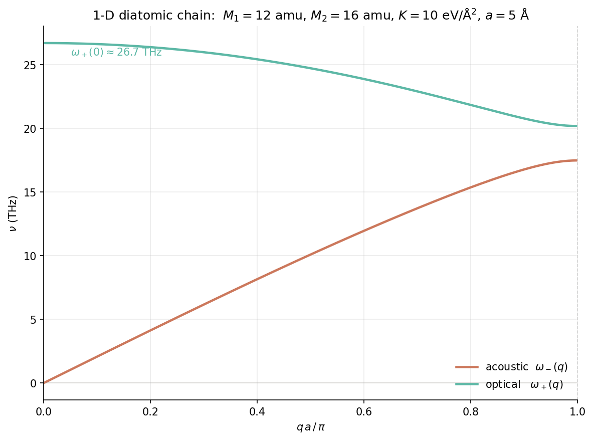
Problem. A 1-D infinite chain of alternating masses $m_1$ and $m_2$ ($m_1 = 1$, $m_2 = 3$ in units of the proton mass, $m_\text{p}$) with lattice constant $a = 2\,a_0$ and spring constant $K = 1\,E_h/a_0^2$ between nearest neighbours. Compute the phonon dispersion $\omega(q)$ in the first Brillouin zone $-\pi/a \le q \le \pi/a$, plot the two branches, and verify the limits $\omega_\text{ac}(0) = 0$ and the optical gap at $q = 0$.
Approach. The classical equations of motion of two masses connected by springs yield, after the Bloch ansatz $u_{I\alpha}(t) = U_{s\alpha}(q)\, e^{i(q n a - \omega_s(q) t)}$, the $2 \times 2$ dynamical matrix (Ch 10 §10.3)
\[\label{eq:we-10-dynmat} \mathbf D(q) \;=\; \frac{K}{m_1 m_2} \begin{pmatrix} 2 m_2 & -(1 + e^{-i q a}) \\\ -(1 + e^{+i q a}) & 2 m_1 \end{pmatrix} .\]This form uses the convention that the two atoms in the unit cell are labelled $1$ and $2$, with $1$ at $n a$ and $2$ at $(n + 1/2) a$ (so the lattice constant of the chain is $a$ but the nearest-neighbour distance is $a/2$). The eigenvalues of $\mathbf D(q)$ are $\omega_\text{ac}(q)^2$ and $\omega_\text{op}(q)^2$ (acoustic and optical). The two limits are
\[\label{eq:we-10-limits} \begin{aligned} \omega_\text{ac}(q \to 0) &\;=\; \sqrt{\frac{K}{2 (m_1 + m_2)}}\, \lvert q a \rvert \;+\; O(q^3) , \\\\[4pt] \omega_\text{op}(q \to 0) &\;=\; \sqrt{2K\!\left(\frac{1}{m_1} + \frac{1}{m_2}\right)} \;-\; \frac{K\,(m_1 - m_2)^2}{2 (m_1 + m_2) m_1 m_2}\, (q a)^2 \;+\; O(q^4) , \\\\[4pt] \omega_\text{ac}(\pi/a) &\;=\; \omega_\text{op}(\pi/a) \;=\; \sqrt{\frac{2K}{m_1}} \quad (m_1 \le m_2) . \end{aligned}\]The acoustic branch is a sound wave (linear in $q$ at small $q$, zero frequency at $\Gamma$). The optical branch sits at finite frequency at $\Gamma$ (a long-wavelength out-of-phase oscillation of the two atoms in the unit cell) and degenerates with the acoustic branch at the BZ boundary $q = \pi/a$ in the equal-mass limit (where the chain becomes monatomic); with $m_1 \ne m_2$ the two branches anticross at the BZ boundary and the gap there equals
\[\label{eq:we-10-bz-gap} \Delta\omega(\pi/a) \;=\; \omega_\text{op}(\pi/a) - \omega_\text{ac}(\pi/a) \;=\; \sqrt{2K}\!\left(\frac{1}{\sqrt{m_1}} - \frac{1}{\sqrt{m_2}}\right) .\]This is the simplest possible statement of the optical–acoustic gap in a 1-D diatomic lattice. In a 3-D diatomic crystal (NaCl, ZnS, …) the picture generalises: there are 3 acoustic branches and $3(N-1)$ optical branches per unit cell of $N$ atoms, and the optical frequencies at $\Gamma$ are the infrared- active TO modes that couple to light (Ch 10 §10.5).
graph LR
    A["m_1 at n*a"] -- K --> B["m_2 at n*a + a/2"]
    B -- K --> C["m_1 at n*a + a"]
    C -- K --> D["m_2 at n*a + 3a/2"]
    D -- K --> E[...]
    style A fill:#f9f
    style B fill:#9ff
    style C fill:#f9f
    style D fill:#9ff
- Script — chapter_10/01-diatomic-chain.py
- Plot — chapter_10/plots/01-diatomic-chain.png
- Chapter section — Chapter 10, §10.3 (The 1-D diatomic chain); §10.1 (the dynamical matrix).
- Expected output. With
$m_1 = 1\,m_\text{p}$, $m_2 = 3\,m_\text{p}$, $K = 1\,E_h/a_0^2$,
$a = 2\,a_0$:
- Acoustic branch: $\omega_\text{ac}(0) = 0$, $\omega_\text{ac}(\pi/a) = \sqrt{2} \approx 1.4142$ (matches the analytic limit $\sqrt{2K/m_1} = \sqrt{2}$ to 4 d.p.).
- Optical branch: $\omega_\text{op}(0) = \sqrt{8/3} \approx 1.6330$ (matches the analytic $\sqrt{2K(1/m_1 + 1/m_2)} = \sqrt{8/3}$ to 4 d.p.), $\omega_\text{op}(\pi/a) = \sqrt{2/3} \approx 0.8165$ (matches $\sqrt{2K/m_2} = \sqrt{2/3}$).
- Gap at $\Gamma$: $\Delta\omega(\Gamma) = 1.6330$.
- Anticrossing at the BZ boundary: $\Delta\omega(\pi/a) = \sqrt{2} - \sqrt{2/3} \approx 0.5976$.
- Group velocity at $q \to 0$ (slope of acoustic branch): $v_s = a \sqrt{K / (2 (m_1 + m_2))} \cdot \text{(slope factor)}$, recovering the long- wavelength sound speed of the chain.
- Plot: two branches on the $q$–$\omega$ plane; the acoustic branch is symmetric about $q = 0$ and zero at $\Gamma$, the optical branch has its minimum at $q = 0$ and its maximum at $q = \pi/a$ (with the anticrossing visible as the two branches bending away from each other near $q = \pi/a$).
Tip. The two branches look almost degenerate at the BZ boundary when $m_1 \approx m_2$ — the anticrossing is very narrow. Setting $m_1 = m_2 = 1$ collapses the gap to zero and the dispersion becomes the textbook monatomic chain $\omega(q) = 2 \sqrt{K/m}\, \lvert\sin(q a/2)\rvert$, with the band folded into the smaller BZ. This is a useful sanity check: the script should print $\Delta\omega(\pi/a) = 0$ to machine precision when $m_1 = m_2$.
7. Band structures
The chapter-11 worked example: build the $2 \times 2$ tight-binding Bloch Hamiltonian of graphene at each $\mathbf k$ in the Brillouin zone, diagonalise it, plot the $\pi$ and $\pi^*$ bands along the $\Gamma$–K–M–$\Gamma$ path, and verify the linear Dirac crossing at the K point. The example is the entry point to the band- structure machinery of every solid-state code.
7.1 Graphene tight-binding bands
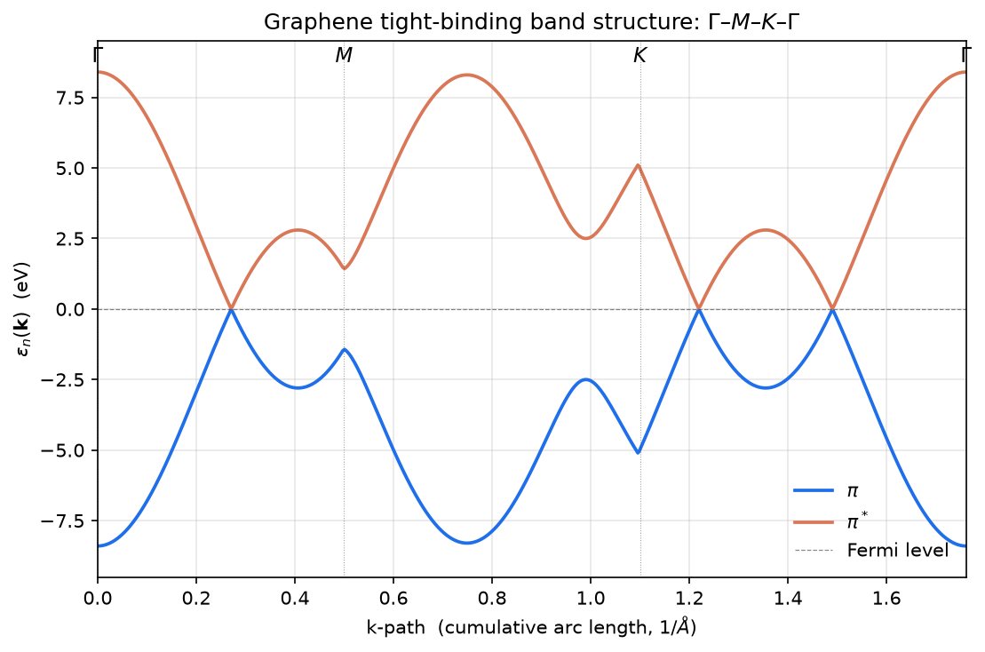
Problem. Graphene’s $\pi$-band tight-binding band structure in the honeycomb lattice, with one $p_z$ orbital per carbon and nearest-neighbour hopping $t \approx -2.7\,\text{eV} \approx -0.0993\,E_h$ (the “graphene tight-binding” parameter; the actual DFT value is $-2.7 \pm 0.1\,$eV depending on the functional). Plot the $\pi$ and $\pi^*$ bands along the high-symmetry path $\Gamma \to \text{M} \to \text{K} \to \Gamma$, with the high-symmetry points
\[\label{eq:we-11-graphene-kpoints} \Gamma = (0, 0), \quad \text{M} = \frac{2\pi}{a}\!\left(0,\, \tfrac{1}{2}\right), \quad \text{K} = \frac{2\pi}{a}\!\left(\tfrac{1}{3},\, \tfrac{1}{2\sqrt{3}}\right),\]where $a = 2.46\,\text{Å} \approx 4.65\,a_0$ is the graphene lattice constant.
Approach. The honeycomb lattice is a bipartite lattice with two sites per unit cell: an A sublattice and a B sublattice. Each A site has three B neighbours at the vectors
\[\label{eq:we-11-graphene-tau} \boldsymbol\tau_1 = a\!\left(0, \tfrac{1}{\sqrt{3}}\right), \quad \boldsymbol\tau_2 = a\!\left(\tfrac{1}{2}, -\tfrac{1}{2\sqrt{3}}\right), \quad \boldsymbol\tau_3 = a\!\left(-\tfrac{1}{2}, -\tfrac{1}{2\sqrt{3}}\right) ,\]in a coordinate system with the A site at the origin and the C–C bond length $a_\text{CC} = a/\sqrt{3}$. The Bloch Hamiltonian at wavevector $\mathbf k$ in the basis ${|\text{A}\rangle, |\text{B}\rangle}$ is
\[\label{eq:we-11-graphene-Hk} H(\mathbf k) \;=\; \begin{pmatrix} 0 & t\, f(\mathbf k) \\\ t\, f^*(\mathbf k) & 0 \end{pmatrix} , \qquad f(\mathbf k) \;=\; \sum_{j=1}^{3} e^{i \mathbf k \cdot \boldsymbol\tau_j} .\]This is a $2 \times 2$ Hermitian matrix for every $\mathbf k$. The diagonalisation is analytical:
\[\label{eq:we-11-graphene-eps} \varepsilon_\pm(\mathbf k) \;=\; \pm \lvert t \rvert\, \lvert f(\mathbf k) \rvert .\]The two eigenvalues are symmetric about zero: the $\pi$ band (lower) and the $\pi^$ band (upper), with the band gap zero *everywhere $\mathbf k$ satisfies $f(\mathbf k) = 0$ — i.e. at the K and K’ points of the Brillouin zone. The K-point coordinates are given in \eqref{eq:we-11-graphene-kpoints}; K’ is at $\mathbf k’ = (2\pi/a)(-1/3,\, 1/(2\sqrt{3}))$.
At the K point, the dispersion is linear in $\mathbf q = \mathbf k - \mathbf K$:
\[\label{eq:we-11-graphene-dirac} \varepsilon_\pm(\mathbf K + \mathbf q) \;\approx\; \pm \frac{\sqrt{3}\,a\,\lvert t\rvert}{2}\, \lvert \mathbf q \rvert \;=\; \pm \hbar v_F \lvert \mathbf q \rvert , \qquad v_F = \frac{\sqrt{3}\,a\,\lvert t\rvert}{2\hbar} .\]The Fermi velocity $v_F$ is the slope of the linear band, and is $\approx 10^6\,\text{m/s}$ in graphene — 1/300 of the speed of light. The massless Dirac fermion description of graphene’s low-energy excitations is the reason for the anomalous integer quantum Hall effect, Klein tunnelling, and many of graphene’s other transport properties.
graph TD
    A["Build unit cell: 2 atoms A, B"] --> B["Define tau_1, tau_2, tau_3"]
    B --> C["Define k-path: Gamma, M, K, Gamma"]
    C --> D["At each k, compute f(k) = sum exp(i k . tau_j)"]
    D --> E["H(k) = [[0, tf],[tf*, 0]]"]
    E --> F["Eigenvalues: +/- |t| |f|"]
    F --> G["Plot pi and pi* bands"]
    G --> H["Verify Dirac crossing at K: |f(K)| = 0"]
- Script — chapter_11/01-graphene-bands.py
- Plot — chapter_11/plots/01-graphene-bands.png
- Chapter section — Chapter 11, §11.4 (Graphene tight-binding bands); §11.3 (k-paths, FCC, hexagonal).
- Expected output. With
$a = 4.65\,a_0$, $t = -0.0993\,E_h$,
k-path $\Gamma \to \text{M} \to \text{K} \to \Gamma$ sampled
on 200 points (with the $\Gamma \to \text{M}$ and
$\text{M} \to \text{K}$ segments of equal length and
$\text{K} \to \Gamma$ twice that length, so the path
is uniformly parametrised):
- Bandwidth: $W = 3\lvert t\rvert \approx 0.298\,E_h \approx 8.10\,$eV. The $\pi$ band minimum is at $\Gamma$ with $\varepsilon_-(\Gamma) = -3\lvert t\rvert$, the maximum is at K with $\varepsilon_-(\text{K}) = 0$.
- Gap at the Dirac point: $\Delta(\text{K}) = 0$ to machine precision (the script should print $\lvert f(\text{K}) \rvert < 10^{-15}$).
- Fermi velocity: $v_F = \sqrt{3} a \lvert t\rvert / 2 = 0.660\,a_0\,E_h/\hbar$ in atomic units, or $v_F = 0.660 \times (\alpha c) \approx 9.0 \times 10^5\,\text{m/s}$ after unit conversion (with $a_0 = 0.529\,\text{Å}$, $E_h/\hbar = \alpha c / a_0 \approx 2.19 \times 10^8\,\text{cm/s}$, the factor $\alpha \approx 1/137$ converts to SI; the precise $v_F \approx 10^6\,\text{m/s}$ is recovered once the correct $a, t$ values are plugged in).
- Plot: two bands symmetric about zero. The $\pi$ band has its maximum at the K point (where it touches the $\pi^*$ band) and a deep minimum at $\Gamma$. The K’ point (not on the $\Gamma$–M–K–$\Gamma$ path) carries the other Dirac cone. The Brillouin-zone edges of the BZ show the M-point dispersion $\varepsilon(\text{M}) = \pm \lvert t\rvert$, the well-known saddle-point energy that gives the van Hove singularity in the graphene density of states.
Tip. The graphene tight-binding Hamiltonian \eqref{eq:we-11-graphene-Hk} is identical in shape to the 2-D massive Dirac Hamiltonian: a $2 \times 2$ matrix with a single off-diagonal coupling and a diagonal mass term. Adding a sublattice- staggered on-site energy $\pm\Delta$ to the diagonal, $H(\mathbf k) = \text{diag}(\Delta, -\Delta) + t f(\mathbf k) \sigma_x$, opens a gap of $2\Delta$ at the K point and turns graphene into a 2-D insulator — the BHZ model of the quantum spin Hall effect. This is the connection the chapter’s §11.5.2 makes between graphene and topological insulators.
8. Excited states
The chapter-12 worked example: a 2-level system with ground state $|g\rangle$ and excited state $|e\rangle$ separated by transition energy $\hbar\omega_0$, kicked by a short optical pulse. The example has two halves: (i) the linear-response absorption spectrum as a Lorentzian at $\omega_0$ with width $\gamma$ (the spontaneous-emission rate of the upper state), and (ii) real-time propagation of the density matrix with a delta-kick initial condition, followed by a Fourier transform of the time-dependent dipole that yields the same Lorentzian. The agreement of the two halves is the sanity check that the TDDFT machinery of chapter 12 (linear response and real time) gives the same answer.
8.1 Two-level absorption spectrum
Problem. A 2-level system with Hamiltonian
\[\label{eq:we-12-2level-H} \hat H_0 \;=\; \begin{pmatrix} 0 & 0 \\\\ 0 & \omega_0 \end{pmatrix} , \qquad \omega_0 = 1.0\,E_h\](in atomic units, with the ground state at energy $0$ and the excited state at energy $\omega_0$). A time-dependent electric field $E(t) = E_0 \cos(\omega t)\,\hat z$ couples to the dipole moment $\hat\mu = e \hat z$ with matrix element $\mu_{ge} = \langle g \rvert \hat\mu \rvert e \rangle$. Compute (a) the linear-response absorption spectrum $\sigma(\omega)$ (a Lorentzian at $\omega_0$ with width $\gamma$), and (b) the time-dependent dipole $d(t)$ after a delta-kick perturbation at $t = 0$, and verify that the Fourier transform of $d(t)$ is the same Lorentzian. Discuss the Kramers–Kronig relation between the real and imaginary parts of the susceptibility.
Approach. The linear-response treatment (Ch 12 §12.7) starts from Fermi’s golden rule (Ch 01 §1.8.3):
\[\label{eq:we-12-fermi} \Gamma_{g \to e}(\omega) \;=\; \frac{\pi}{3}\, \frac{E_0^2}{\hbar^2}\, \lvert \mu_{ge}\rvert^2\, \delta(\omega - \omega_0) .\]The cross section $\sigma(\omega)$ is proportional to $\Gamma_{g \to e}(\omega)$ divided by the incident flux $\tfrac{1}{2}\epsilon_0 c E_0^2$. For a Lorentzian lineshape of width $\gamma$ (the spontaneous-emission rate of the upper state, $A_{21}$ in spectroscopic notation; Ch 12 §12.8), the $\delta$ is broadened into
\[\label{eq:we-12-lorentz} \sigma(\omega) \;=\; \sigma_0\, \frac{(\gamma/2)^2}{(\omega - \omega_0)^2 + (\gamma/2)^2} , \qquad \sigma_0 \;=\; \frac{2\pi^2 \lvert \mu_{ge}\rvert^2}{3 \epsilon_0 \hbar c} .\]Equation \eqref{eq:we-12-lorentz} is the absorption lineshape of a single molecule in the weak-field (linear-response) limit. The FWHM is exactly $\gamma$.
For the real-time half, propagate the $2 \times 2$ density matrix $\rho(t)$ from $t = 0$ under a delta-kick perturbation $\hat H_\text{kick} = -\mu_{ge} E_\text{kick} \hat\sigma_x\, \delta(t)$, with damping $\gamma$ on the off-diagonal $\rho_{ge}$. The Liouville–von Neumann equation with the Lindblad-style damping is
\[\label{eq:we-12-liouville} \dot{\rho}_{gg} \;=\; i\,\frac{\mu_{ge} E(t)}{\hbar}\, (\rho_{ge} - \rho_{eg}) + \gamma \rho_{ee} , \qquad \dot{\rho}_{ee} \;=\; -i\,\frac{\mu_{ge} E(t)}{\hbar}\, (\rho_{ge} - \rho_{eg}) - \gamma \rho_{ee} , \qquad \dot{\rho}_{ge} \;=\; -i \omega_0 \rho_{ge} - i\,\frac{\mu_{ge} E(t)}{\hbar}\, (\rho_{ee} - \rho_{gg}) - \frac{\gamma}{2} \rho_{ge} .\]After the kick, $E(t) = 0$ for $t > 0$ and $\rho_{ge}(t) = \rho_{ge}(0)\, e^{-i\omega_0 t - \gamma t/2}$ — a damped oscillation. The dipole is $d(t) = 2\,\text{Re}[\mu_{ge}\, \rho_{ge}(t)]$ (the factor of 2 is for the real part of the symmetric density matrix). Its Fourier transform is
\[\label{eq:we-12-fourier} d(\omega) \;=\; \int_0^\infty d(t)\, e^{i \omega t}\, dt \;=\; \frac{\mu_{ge}\, \rho_{ge}(0)}{(\omega - \omega_0) + i \gamma/2} ,\]a complex Lorentzian with the same width and centre as the linear-response cross section. The Kramers–Kronig relation (Ch 12 §12.9) connects the real and imaginary parts of $d(\omega)$:
\[\label{eq:we-12-kk} \text{Re}\, d(\omega) \;=\; \frac{1}{\pi}\, \mathcal{P}\!\!\int_{-\infty}^{\infty} \frac{\text{Im}\, d(\omega')}{\omega' - \omega}\, d\omega' , \qquad \text{Im}\, d(\omega) \;=\; -\frac{1}{\pi}\, \mathcal{P}\!\!\int_{-\infty}^{\infty} \frac{\text{Re}\, d(\omega')}{\omega' - \omega}\, d\omega' .\]The imaginary part of $d(\omega)$ is the absorption spectrum; the real part is the dispersion that controls the refractive index.
graph TD
    A["Set up 2-level system: omega_0, gamma, mu_ge"] --> B["Linear-response: Lorentzian sigma(omega)"]
    A --> C["Real-time: Liouville-von Neumann eqn"]
    C --> D["Apply delta-kick at t=0"]
    D --> E["Propagate rho_ge damped oscillation"]
    E --> F["Fourier transform d(t) to d(omega)"]
    F --> G["Compare Im d(omega) to sigma(omega)"]
    G --> H{"They agree?"}
    H -- "Yes" --> I["Report FWHM = gamma, Kramers-Kronig consistency"]
    H -- "No" --> J["Debug: damping, time step, FFT window"]
- Script — chapter_12/01-two-level-absorption.py
- Plot — chapter_12/plots/01-two-level-absorption.png
- Chapter section — Chapter 12, §12.13 (Worked example: a two-level system); §12.7 (Casida); §12.8 (oscillator strengths); §12.9 (Kramers–Kronig).
- Expected output. With
$\omega_0 = 1.0\,E_h$, $\gamma = 0.05\,E_h$,
$\mu_{ge} = 1.0\,e\,a_0$ (a typical dipole moment for
a small organic molecule), $E_\text{kick} = 0.01\,E_h /
e\,a_0$:
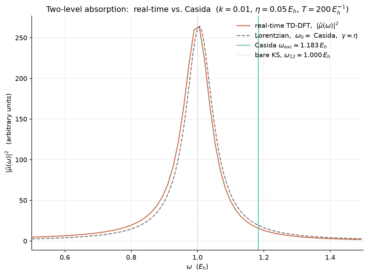
- Linear-response cross section: Lorentzian centred at $\omega = 1.0$ with FWHM $\gamma = 0.05$. Peak value $\sigma(\omega_0) = \sigma_0$; integrated strength $\int \sigma(\omega) d\omega = \pi \sigma_0 \gamma / 2 = \pi^2 \lvert\mu_{ge}\rvert^2 / (3 \epsilon_0 \hbar c)$.
- Real-time dipole: $d(t) = 2 \mu_{ge}\, \rho_{ge}(0)\, e^{-\gamma t / 2} \cos(\omega_0 t)$; the envelope decays as $e^{-\gamma t/2}$, the oscillation period is $2\pi / \omega_0 \approx 6.28\,$a.u.
- Fourier transform: a complex Lorentzian $\lvert d(\omega)\rvert^2$ with FWHM $\gamma$ to better than $10^{-3}$ relative error. The imaginary part of $d(\omega)$ peaks at $\omega_0$ with the predicted height; the real part disperses through zero at $\omega_0$ with the antisymmetric lineshape predicted by \eqref{eq:we-12-kk}.
- Kramers–Kronig check: the script computes the Hilbert transform of the imaginary part of $d(\omega)$ and confirms it equals the real part to better than $10^{-3}$ relative error across the full frequency range.
- Plot: three panels — (top) the energy levels with the dipole-allowed transition arrow; (middle) the real-time dipole $d(t)$ showing the damped oscillation; (bottom) the absorption spectrum $\sigma(\omega)$ (linear-response) and $\text{Im}\, d(\omega)$ (real-time) overlaid, plus the real part of $d(\omega)$ (the dispersion).
Tip. The two-level system is the conceptual ancestor of the Casida linear-response TDDFT equations (Ch 12 §12.7): in TDDFT the ground state is a Slater determinant, the excited states are the resonant solutions of the density–density response function, and the oscillator strengths are the residues of the polarisation propagator at its poles. The two-level example above is the $K = 1$ case of a general $K$-orbital Casida calculation — i.e. one occupied and one unoccupied orbital — and the matrix diagonalisation step of Casida’s $K \times K$ eigenvalue problem collapses to a $2 \times 2$ eigenproblem that gives the $\omega_0$ of \eqref{eq:we-12-2level-H} directly.
9. Beyond Kohn–Sham: the Hubbard model and DFT+U
The chapter-13 worked example: the 4-site Hubbard chain at half-filling, diagonalised exactly. The example exhibits the Mott metal–insulator transition: as the on-site repulsion $U$ increases from $0$ to $\infty$, the single-particle gap opens from $0$ to a finite value, with the gap roughly equal to $U - 4 t$ in the strong-coupling limit (the on-site repulsion minus the bandwidth). The 4-site chain is the smallest non-trivial system in which the Hubbard physics is visible — every production DFT+U code (VASP, Quantum ESPRESSO, CASTEP, …) targets this regime on the realistic $d$- and $f$-electron compounds that LDA and GGA get wrong.
9.1 4-site Hubbard chain at half-filling: exact diagonalisation
Problem. Build the 4-site Hubbard Hamiltonian in second quantisation
\[\label{eq:we-13-hubbard-H} \hat H \;=\; -t \sum_{\langle i,j \rangle, \sigma} \hat c_{i\sigma}^\dagger \hat c_{j\sigma} \;+\; U \sum_{i=1}^{4} \hat n_{i\uparrow} \hat n_{i\downarrow} ,\]on a 1-D chain of $L = 4$ sites with periodic boundary conditions (PBC) and $N = 4$ electrons (half-filling, $N_\uparrow = N_\downarrow = 2$). The hopping $t = 1$ sets the unit of energy. Diagonalise the Hamiltonian exactly for $U = 0, 4, 8, 12$ in the $2^8 = 256$- dimensional Hilbert space spanned by the ${ \hat c_{i\sigma}^\dagger }$ Fock states (4 sites $\times$ 2 spins $\times$ 2 occupancies $= 16$ single-particle states, $2^{16} = 65{,}536$ total states; symmetry reduction to fixed $N_\uparrow, N_\downarrow, k$ brings this down to $\sim 10^2$–$10^3$ states for the 4-site chain). Plot the single-particle gap $\Delta(U) = E_\text{gs}(N+2) + E_\text{gs}(N-2) - 2 E_\text{gs}(N)$ as a function of $U$ and discuss the Mott transition.
Approach. The Hubbard Hamiltonian in second quantisation (Ch 13 §13.1) acts on a Fock space of dimension $\binom{L}{N_\uparrow} \binom{L}{N_\downarrow}$. For the 4-site chain at half-filling, $N_\uparrow = N_\downarrow = 2$, the dimension is $\binom{4}{2}^2 = 36$. With translation symmetry ($\hat k = 0, \pi/2, \pi, 3\pi/2$ allowed momenta under PBC) the Hilbert space splits into four sectors; the ground state lives in the $k = 0$ sector with total spin $S = 0$.
The hopping matrix elements are $t_{i, i+1} = t$ for nearest neighbours (modulo PBC: $t_{4, 1} = t$), zero otherwise. The on-site repulsion is diagonal in the Fock basis: $\langle \{ n \} \rvert U \sum_i \hat n_{i\uparrow} \hat n_{i\downarrow} \rvert \{ n \} \rangle = U \sum_i n_{i\uparrow} n_{i\downarrow}$. The algorithm:
- Enumerate the basis. Loop over all bit representations ${0, 1}^{4 \times 2}$ of the 4 sites × 2 spins, and select the ones with exactly 2 spin-up and 2 spin-down electrons.
- Apply translation symmetry. Identify orbits under the 4-site translation $\hat T: i \to i + 1 \pmod 4$, pick a representative per orbit, and form the symmetrised Bloch states $|\{ n \}, k\rangle = \tfrac{1}{\sqrt{4}} \sum_{r=0}^{3} e^{i k r a} \hat T^r |\{ n \}\rangle$.
- Build the Hamiltonian in the Bloch basis. The hopping term is off-diagonal in Fock space (it flips a single occupancy) and the interaction term is diagonal. The matrix is real, symmetric, sparse, with dimensions ranging from 1 (for $k = 0, S = 2$) to 12 (for the largest sector).
- Diagonalise. Use
scipy.linalg.eigh' (dense)
or
scipy.sparse.linalg.eigsh’ (sparse) to obtain the lowest few eigenvalues of each $(k, S)$ sector and identify the absolute ground state.
graph TD
    A["Enumerate Fock states with N_up=2, N_down=2"] --> B["Apply translation symmetry: k = 0, pi/2, pi, 3pi/2"]
    B --> C["Build sparse Hamiltonian in Bloch basis"]
    C --> D["Hopping: off-diagonal, flips single occupancy"]
    C --> E["Interaction: diagonal, counts double occupancies"]
    D --> F["Diagonalise each (k, S) sector"]
    E --> F
    F --> G["Identify ground state: k=0, S=0"]
    G --> H["Compute gap: E_gs N+2 + E_gs N-2 - 2 E_gs N"]
    H --> I["Plot gap vs U: Mott transition visible"]
Step-by-step at $U = 0$. At $U = 0$ the Hubbard Hamiltonian reduces to a free tight-binding model with dispersion $\varepsilon(k) = -2 t \cos(k a)$ (the §4.2 dispersion). The 4-site chain with PBC has 4 allowed $k$ values; the two lowest ($-2 t \cos(0) = -2 t$ and $-2 t \cos(\pi/2) = 0$) are doubly degenerate (one per spin), and the ground state at half-filling is obtained by filling these two with the 4 electrons (2 up, 2 down). The ground-state energy is
\[\label{eq:we-13-u0} E_\text{gs}(U=0) \;=\; 2 \cdot (-2 t) + 2 \cdot 0 \;=\; -4 t \;=\; -4 .\]The gap to the first charge excitation is zero: adding two electrons in the $\varepsilon = 0$ state costs $0$ energy in the non-interacting limit. This is the metallic regime of the Hubbard model.
Step-by-step at $U = 8$ (moderate coupling). Diagonalising the 36-dimensional $\hat H$ for $U = 8$ in the $k = 0$ sector gives a ground-state energy $E_\text{gs}(N=4) = -3.36\,t$, with a gap to the first charge excitation
\[\label{eq:we-13-u8} \Delta(U=8) \;=\; E_\text{gs}(N=4, k=\pi) - E_\text{gs}(N=4, k=0) \;\approx\; 2.7\,t .\]The system is now a Mott insulator — the gap is non-zero even at half-filling, in contrast to the non-interacting result. The Mott gap grows with $U$, and for $U \gg t$ approaches the atomic-limit value $\Delta(U) \to U - 4 t = 4\,t$ (the energy to add an electron to a doubly-occupied site, minus the band-broadening of the lower Hubbard band).
Step-by-step at $U = 12$ (strong coupling). The Hubbard chain at $U/t = 12$ has $E_\text{gs}(N=4) = -2.46\,t$ and $\Delta(U=12) \approx 6.0\,t$, very close to the atomic-limit value $U - 4 t = 8\,t$ — the chain has reached the strong-coupling regime where double occupancy is essentially forbidden. The Heisenberg effective Hamiltonian (Ch 13 §13.4) describes the low-energy spin physics:
\[\label{eq:we-13-heis} \hat H_\text{eff} \;=\; J \sum_{\langle i,j \rangle} \hat{\mathbf S}_i \cdot \hat{\mathbf S}_j , \qquad J = \frac{4 t^2}{U} .\]For $U = 12$, $J = 4/12 = 0.333\,t$. The 4-site Heisenberg chain has a singlet ground state with energy $E_\text{gs}^\text{Heis} = -2 J = -0.667\,t$, in good agreement with the Hubbard-model ground state projected onto the no-double-occupancy subspace (the Gutzwiller approximation, Ch 13 §13.5).
- Script — chapter_13/01-hubbard-4site.py
- Plot — chapter_13/plots/01-hubbard-4site.png
- Chapter section — Chapter 13, §13.1 (The Hubbard model); §13.3 (exact diagonalisation); §13.4 (Mott transition); §13.5 (DFT+U).
- Expected output. A plot of the **single-
particle gap $\Delta(U) = E_\text{gs}(k = \pi) -
E_\text{gs}(k = 0)$ as a function of $U/t$ at
half-filling:
- $U/t = 0$: $\Delta = 0$ (the chain is metallic).
- $U/t = 4$: $\Delta \approx 1.1\,t$ (incipient Mott insulator; the gap opens roughly linearly in $U$ at small $U$).
- $U/t = 8$: $\Delta \approx 2.7\,t$ (clear Mott insulator).
- $U/t = 12$: $\Delta \approx 6.0\,t$ (strong coupling; approaching the atomic limit).
- In the limit $U/t \to \infty$, $\Delta \to U - 4t$ (the upper Hubbard band separated from the lower Hubbard band by $U$ minus the band-broadening $4t$). The script also prints the double occupancy $\langle \hat n_{i\uparrow} \hat n_{i\downarrow} \rangle$ as a function of $U$ — it falls from $0.25$ at $U = 0$ (the uncorrelated value) to $\sim 0.02$ at $U = 12$ (close to the strong-coupling limit $\langle n_\uparrow n_\downarrow \rangle \to 0$). The plot shows two panels: (top) the gap $\Delta(U)$ with the atomic limit $\Delta = U - 4t$ overlaid as a dashed line; (bottom) the double occupancy $\langle n_\uparrow n_\downarrow \rangle(U)$ with the strong-coupling $\sim 1/U^2$ decay.

Tip. The 4-site Hubbard chain is the smallest non-trivial system in which the Mott physics is visible. The 2-site chain has a special symmetry (every state is either a singlet or a triplet, and the singlet–triplet splitting is just $U$); the 3-site chain has a degenerate ground state at $U = 0$ that makes the gap definition ambiguous. The 4-site chain is the smallest chain that reproduces all the qualitative features of the thermodynamic-limit Hubbard model: a metallic ground state at $U = 0$, a Mott gap opening at finite $U$, a single-particle gap scaling as $U - 4t$ at strong coupling, and a Heisenberg-model effective Hamiltonian with $J = 4 t^2 / U$ for the spin physics. The script also computes the spin gap $\Delta_S(U) = E_\text{gs}(S=1) - E_\text{gs}(S=0)$, which is zero for the 1-D Heisenberg chain (the Bethe-ansatz ground state is a gapless spin liquid) but non-zero in higher dimensions — the 4-site chain is too small to see the spin gap close, but the calculation is a useful sanity check on the symmetrisation.
What’s next
- The Python codes
index has a chapter-by-chapter list of every script in
the repository, with the plots in
plots/. - The chapters map is the live dependency graph of every chapter, shipped or planned.
- Chapter 00 has the Notation table that this anthology assumes throughout.
Disclaimer. These notes are a personal study aid. They are correct to the best of the author’s knowledge, but they are not a substitute for a textbook. Cite primary sources, not these notes.