Chapter 06 — Basis sets
The Fock and Kohn–Sham operators live in an infinite-dimensional Hilbert space. We can only diagonalise finite matrices. A basis set is the bridge between the two — and the choice of bridge is what every practical DFT calculation rides on.
By the end of chapter 05 we had reduced the electronic-structure problem to a one-body eigenvalue equation for the Kohn–Sham (or Fock) orbitals. Both $\hat F \phi_i = \varepsilon_i \phi_i$ (chapter 03) and $\hat H_\text{KS} \phi_i = \varepsilon_i \phi_i$ (chapter 04) are differential equations in $\mathbb R^3$ whose unknown is a function. A computer cannot store a function; it can only store a finite array of numbers. The standard trick is to expand each orbital in a chosen, finite set of $K$ known functions ${\chi_\mu}{\mu=1}^K$ — the basis set — so that the orbital is encoded by $K$ expansion coefficients. The differential eigenvalue equation then collapses to a matrix eigenvalue problem. This chapter explains which ${\chi\mu}$ are used in practice, why each family was invented, and what numerical price each charges.
6.1 The claim — Roothaan–Hall
For a closed-shell molecule, expanding each spatial orbital in the same $K$ basis functions ${\chi_\mu}$,
\[\label{eq:ch-06-basis-expansion} \phi_i(\mathbf r) \;=\; \sum_{\mu=1}^{K} C_{\mu i}\, \chi_\mu(\mathbf r) ,\]turns the Fock equation $\hat F \phi_i = \varepsilon_i \phi_i$ into the Roothaan–Hall matrix equation
\[\label{eq:ch-06-roothaan-hall} \mathbf F\, \mathbf C \;=\; \mathbf S\, \mathbf C\, \boldsymbol\varepsilon ,\]where $\mathbf F$, $\mathbf S$, $\mathbf C$ are $K \times K$ matrices and $\boldsymbol\varepsilon$ is the diagonal matrix of orbital energies. The matrix elements are
\[\label{eq:ch-06-fock-overlap} F_{\mu\nu} \;=\; \langle \chi_\mu \rvert \hat F \rvert \chi_\nu \rangle , \qquad S_{\mu\nu} \;=\; \langle \chi_\mu \rvert \chi_\nu \rangle .\]Derivation. Substitute \eqref{eq:ch-06-basis-expansion} into $\hat F \phi_i = \varepsilon_i \phi_i$,
\[\hat F \sum_\mu C_{\mu i} \chi_\mu = \varepsilon_i \sum_\mu C_{\mu i} \chi_\mu .\]Project both sides on $\chi_\nu$ by multiplying with $\chi_\nu^*$ and integrating over $\mathbf r$:
\[\sum_\mu C_{\mu i}\, \underbrace{\langle \chi_\nu \rvert \hat F \rvert \chi_\mu \rangle}_{F_{\nu\mu}} \;=\; \varepsilon_i \sum_\mu C_{\mu i}\, \underbrace{\langle \chi_\nu \rvert \chi_\mu \rangle}_{S_{\nu\mu}} .\]This is the $i$-th column of the matrix equation $\mathbf F \mathbf C = \mathbf S \mathbf C \boldsymbol\varepsilon$. Collecting all $K$ MOs (i.e. all values of $i$) into one matrix gives \eqref{eq:ch-06-roothaan-hall}.
Tip. The basis is in general non-orthogonal, so the right-hand side carries an $\mathbf S$ that the orthonormal $\hat F \phi_i = \varepsilon_i \phi_i$ does not have. This is not a mistake; it is the price of choosing a basis adapted to the physics (atom-centred Gaussians look like atomic orbitals) rather than to the math (an orthonormal basis is mathematically clean but physically unmotivated).
Equation \eqref{eq:ch-06-roothaan-hall} is a generalised eigenvalue problem. `scipy.linalg.eigh(F, S)’ solves it directly; internally it computes $\mathbf X = \mathbf S^{-1/2}$, forms $\mathbf F’ = \mathbf X^\dagger \mathbf F \mathbf X$, diagonalises $\mathbf F’$ (now a standard eigenproblem), and transforms the eigenvectors back via $\mathbf C = \mathbf X \mathbf C’$.
6.2 Why we need a basis
The exact orbital $\phi_i^\text{exact}$ lives in $L^2(\mathbb R^3)$, an infinite-dimensional Hilbert space. Every basis we will meet is a finite subset ${\chi_\mu}_{\mu=1}^K \subset L^2(\mathbb R^3)$ that spans a $K$-dimensional subspace $\mathcal V_K$. The variational principle (chapter 03) says
\[\label{eq:ch-06-variational} E_0^\text{basis}(K) \;\equiv\; \min_{\phi \in \mathcal V_K}\, E[\phi] \;\ge\; E_0^\text{exact} ,\]with equality only in the limit $K \to \infty$ along a sequence of basis sets whose span becomes dense in $L^2(\mathbb R^3)$. The gap between $E_0^\text{basis}(K)$ and $E_0^\text{exact}$ is the basis-set incompleteness error:
\[\label{eq:ch-06-bsie} \Delta E_\text{BSIE}(K) \;\equiv\; E_0^\text{basis}(K) \;-\; E_0^\text{CBS} ,\]where $E_0^\text{CBS}$ is the value at the complete-basis-set limit (CBS, $K \to \infty$). For atom-centred Gaussians on small molecules, a typical empirical rule is that $\Delta E_\text{BSIE}$ falls roughly exponentially with the cardinal number $X$ of the Dunning correlation-consistent family (cc-pVXZ),
\[\label{eq:ch-06-cbs-extrap} E(X) \;\approx\; E^\text{CBS} \;+\; A\, e^{-\alpha X} ,\]which is the formula used to extrapolate to $E^\text{CBS}$ from two or three calculations at $X = D, T, Q$.
Note. The BSIE is one of two approximation errors in any practical calculation. The other is the exchange–correlation functional (chapter 05). A converged DFT energy is only meaningful once both have been pushed to a known tolerance. Quoting a DFT energy without naming the basis is like quoting a price without naming the currency.
6.3 Gaussian-type orbitals (GTOs)
A primitive Cartesian Gaussian centred at $\mathbf A$ with exponent $\alpha$ and angular indices $(\ell_x, \ell_y, \ell_z)$ is
\[\label{eq:ch-06-primitive} g(\mathbf r;\alpha,\mathbf A,\boldsymbol\ell) \;=\; N(\alpha,\boldsymbol\ell)\, (x - A_x)^{\ell_x} (y - A_y)^{\ell_y} (z - A_z)^{\ell_z}\, e^{-\alpha |\mathbf r - \mathbf A|^2} ,\]with $N(\alpha,\boldsymbol\ell)$ chosen so that $\int |g|^2\, d\mathbf r = 1$. The total angular momentum is $\ell = \ell_x + \ell_y + \ell_z$, with $\ell = 0$ called “s-type”, $\ell = 1$ “p-type”, $\ell = 2$ “d-type”, and so on.
For $\ell = 0$ the normalisation collapses to
\[\label{eq:ch-06-norm-s} N(\alpha) \;=\; \left( \frac{2\alpha}{\pi} \right)^{3/4} .\]Why Gaussians and not Slater functions? Slater-type orbitals (STOs) $e^{-\zeta r}$ have the right short-range cusp at the nucleus and the right exponential decay at infinity — properties Gaussians do not share. Yet every production quantum-chemistry code uses Gaussians, because of one critical algebraic identity: the Gaussian product theorem. For two s-primitives at centres $\mathbf A$ and $\mathbf B$ with exponents $\alpha$ and $\beta$,
\[\label{eq:ch-06-gpt} e^{-\alpha |\mathbf r - \mathbf A|^2}\, e^{-\beta |\mathbf r - \mathbf B|^2} \;=\; K_{AB}\, e^{-(\alpha+\beta) |\mathbf r - \mathbf P|^2} ,\]with the Gaussian midpoint $\mathbf P = (\alpha \mathbf A + \beta \mathbf B)/(\alpha+\beta)$ and the prefactor $K_{AB} = \exp!\big[-\alpha\beta/(\alpha+\beta)\, |\mathbf A - \mathbf B|^2\big]$. A two-centre integral has therefore been reduced to a one-centre integral — the integrand is again a Gaussian, located at $\mathbf P$. No such collapse exists for STOs, which is why all four-centre two-electron integrals are tractable in a Gaussian basis and not in a Slater basis.
A contracted Gaussian-type orbital (CGTO) is a fixed linear combination of primitives,
\[\label{eq:ch-06-contraction} \chi_\mu(\mathbf r) \;=\; \sum_{p=1}^{n_\mu} d_{\mu p}\, g(\mathbf r;\alpha_{\mu p},\mathbf A_\mu,\boldsymbol\ell_\mu) ,\]where the contraction coefficients $d_{\mu p}$ and exponents $\alpha_{\mu p}$ are fixed at the moment of designing the basis set, not optimised during the SCF. The contraction $\chi_\mu$ is the one basis function the self-consistent procedure sees; the primitives are implementation detail.
The (ss|ss) two-electron integral
The simplest of the four-centre two-electron integrals is the one between four normalised primitive s-Gaussians (centres $\mathbf A$, $\mathbf B$, $\mathbf C$, $\mathbf D$ and exponents $\alpha,\beta,\gamma,\delta$). Apply \eqref{eq:ch-06-gpt} twice — once to the bra $g_A(\mathbf r_1) g_B(\mathbf r_1)$ and once to the ket $g_C(\mathbf r_2) g_D(\mathbf r_2)$ — to collapse the integrand into a product of two Gaussians at the midpoints $\mathbf P$ and $\mathbf Q$:
\[(AB | CD) = N_A N_B N_C N_D\, K_{AB} K_{CD}\, \int\!\!\int \frac{e^{-(\alpha+\beta)|\mathbf r_1 - \mathbf P|^2}\, e^{-(\gamma+\delta)|\mathbf r_2 - \mathbf Q|^2}} {|\mathbf r_1 - \mathbf r_2|}\, d\mathbf r_1\, d\mathbf r_2 .\]The double integral over the Coulomb kernel can be done analytically (Boys 1950) by inserting the identity $1/r_{12} = (2/\sqrt\pi) \int_0^\infty e^{-s^2 r_{12}^2}\, ds$ and integrating $\mathbf r_1, \mathbf r_2$ as a Gaussian. The result, in normalised form, is
\[\label{eq:ch-06-ssss} (AB | CD) \;=\; \frac{2\pi^{5/2}}{(\alpha+\beta)(\gamma+\delta)\sqrt{\alpha+\beta+\gamma+\delta}}\, K_{AB}\, K_{CD}\, F_0\!\left( \frac{(\alpha+\beta)(\gamma+\delta)}{\alpha+\beta+\gamma+\delta}\, |\mathbf P - \mathbf Q|^2 \right) ,\]where the Boys function
\[\label{eq:ch-06-boys} F_0(t) \;=\; \int_0^1 e^{-t u^2}\, du \;=\; \frac{1}{2}\sqrt{\frac{\pi}{t}}\,\operatorname{erf}(\sqrt{t}) , \qquad F_0(0) = 1 ,\]handles the Coulomb singularity. Every four-centre ERI in quantum chemistry is, after the Gaussian product theorem and McMurchie–Davidson-style recursion in $\boldsymbol\ell$, ultimately a sum of \eqref{eq:ch-06-ssss}-type expressions. This is why GTOs win: they buy analytical ERIs.
6.4 STO-nG — the minimal basis
The cheapest atom-centred basis is the minimal basis: one contracted s-function for each occupied s-shell, one contracted p-shell for each occupied p-shell, and nothing else. For H it is a single 1s; for C it is 1s, 2s, $2p_x$, $2p_y$, $2p_z$ (five functions); for the second row it is nine.
The historical and pedagogical default for a minimal basis is STO-nG (Hehre, Stewart, Pople, 1969): fit each Slater 1s $e^{-\zeta r}$ by a least-squares contraction of $n$ primitive Gaussians,
\[\label{eq:ch-06-sto-fit} \sum_{p=1}^{n} d_p\, g_p(\alpha_p,\,\mathbf 0,\, \boldsymbol 0) \;\approx\; \frac{\zeta^{3/2}}{\sqrt\pi}\, e^{-\zeta r} \quad \text{(in the least-squares sense)} .\]The $n = 3$ case, STO-3G, is the canonical example. The underlying $\zeta = 1.0$ fit for the 1s function (HSP 1969, Table II) is
| $p$ | $\alpha_p$ ($\zeta = 1.0$) | $d_p$ |
|---|---|---|
| 1 | 0.10982 | 0.444635 |
| 2 | 0.40578 | 0.535328 |
| 3 | 2.22766 | 0.154329 |
For a different $\zeta$, the exponents scale as $\alpha_p \to \zeta^2 \alpha_p$ while the $d_p$ are unchanged — a consequence of the Gaussian dimension analysis $\alpha r^2 = (\zeta r)^2 (\alpha/\zeta^2)$. The recommended Pople value for H in molecules is $\zeta = 1.24$, so the H STO-3G exponents actually used in calculations are $\alpha_p \cdot 1.24^2 = 1.5376\, \alpha_p$,
| $p$ | $\alpha_p$ ($\zeta = 1.24$, EMSL default) | $d_p$ |
|---|---|---|
| 1 | 0.168856 | 0.444635 |
| 2 | 0.623913 | 0.535328 |
| 3 | 3.425250 | 0.154329 |
which is the form distributed by the EMSL Basis Set Exchange and consumed directly by every quantum-chemistry code. The worked example in section 6.9 uses this set verbatim.
Warning. STO-3G is a teaching basis. Its absolute errors against the basis-set limit are tens of milli-Hartree, and its predicted bond lengths and frequencies have known, systematic biases. Nobody publishes STO-3G production numbers in 2025. But its small size — two functions for $\rm H_2$, ten for $\rm H_2 O$ — makes it the right basis for a worked example (section 6.9).
6.5 Split-valence: 3-21G, 6-31G, 6-311G
The minimal basis treats the core and the valence the same way — one contracted function per shell. Chemistry happens in the valence, so a small improvement is to leave the core contracted (it barely changes between molecules) and split the valence: replace one valence function by two (or three) of different size, letting the SCF readjust the valence “radius” molecule by molecule.
The Pople split-valence notation is
\[\underbrace{N}_\text{core prims} \text{-} \underbrace{M_1}_\text{inner valence} \underbrace{M_2}_\text{outer valence} \cdots \text{G} ,\]read as: “the core orbital is a single contraction of $N$ primitives; each valence shell is split into one inner function (contraction of $M_1$ primitives) and one outer function (contraction of $M_2$ primitives)”. Examples:
| Basis | Core (per shell) | Valence (per shell) | Cost class |
|---|---|---|---|
| 3-21G | 3 prims, 1 CGTO | (2 + 1) prims, 2 CGTOs | “double-zeta valence” |
| 6-31G | 6 prims, 1 CGTO | (3 + 1) prims, 2 CGTOs | double-zeta valence |
| 6-311G | 6 prims, 1 CGTO | (3 + 1 + 1) prims, 3 CGTOs | “triple-zeta valence” |
For H, which has no core, the basis is purely valence: in 6-31G, H carries 4 primitive s-Gaussians contracted into one “inner” $1s$ (3 prims) and one “outer” $1s’$ (1 prim), so two basis functions per H. In 3-21G it is 3 primitives → two basis functions per H. In 6-311G, three basis functions per H.
Counting basis functions. Add up contracted functions across atoms. For $\rm H_2 O$ in 6-31G:
- O: $1\text{s}$ (core, 1 CGTO) + $2\text{s}$ + $2\text{s}’$ + three $2\text{p}$ + three $2\text{p}’$ = 9 CGTOs
- H: $1\text{s}$ + $1\text{s}’$ = 2 CGTOs
Total $K = 9 + 2 \cdot 2 = 13$ basis functions.
6.6 Polarisation, diffuse, and the cc-pVXZ family
A double-zeta valence basis can resize a $2\text{p}$ orbital on carbon, but it cannot give it the angular flexibility it needs to bend in a bond. For that, add functions of higher angular momentum than the highest occupied shell on each atom:
- on H (highest occupied $\ell = 0$) add a $p$-function,
- on C, N, O (highest occupied $\ell = 1$) add a $d$-function,
- on first-row transition metals (highest occupied $\ell = 2$) add an $f$-function.
These are polarisation functions. Pople’s notation marks them with a star: $6\text{-}31\text{G}^$ adds $d$ on heavy atoms only; $6\text{-}31\text{G}^{**}$ adds $d$ on heavy atoms *and $p$ on H. More polarisation = more flexibility = lower $E_\text{BSIE}$ — but more functions and quartic ERI count.
A complementary direction is to add diffuse functions: primitive Gaussians with very small exponents ($\alpha \sim 0.01$–$0.1$) for the long-range tail of the electron density. Diffuse functions are essential for anions, Rydberg states, hydrogen-bonded systems, and any property that probes the density far from the nuclei (polarisabilities, dipole moments). Pople marks them with a $+$: $6\text{-}31\text{+G}$ adds diffuse $s$ and $p$ on heavy atoms; $6\text{-}31\text{++G}$ also on H.
Correlation-consistent: cc-pVXZ
Dunning’s correlation-consistent family (cc-pVXZ, X = D, T, Q, 5, 6, …) is designed so that each rung adds the functions that recover the next decade of correlation energy. At cardinal number $X$ each atom carries contractions up to angular momentum $\ell = X - 1$ (for first- row atoms; H lags by one):
| Basis | Composition per first-row atom (s, p, d, f, g, …) | $K$ for C |
|---|---|---|
| cc-pVDZ | (3s, 2p, 1d) | 14 |
| cc-pVTZ | (4s, 3p, 2d, 1f) | 30 |
| cc-pVQZ | (5s, 4p, 3d, 2f, 1g) | 55 |
| cc-pV5Z | (6s, 5p, 4d, 3f, 2g, 1h) | 91 |
The augmented variant aug-cc-pVXZ prepends one diffuse function at each angular momentum. The empirical fact that \eqref{eq:ch-06-cbs-extrap} holds for this family is what makes the cc-pVXZ series the de facto path to converged post-HF results.
Note. $X = D, T, Q, 5, 6$ corresponds to “double, triple, quadruple, quintuple, sextuple” zeta — the number of exponents in the contracted valence shells. The label tracks the angular completeness, not just the radial resolution.
6.7 Plane waves
For a periodic system — a crystal, or a molecule placed in a sufficiently large simulation box — the Kohn–Sham orbitals satisfy Bloch’s theorem (we will treat this carefully in chapter 07):
\[\label{eq:ch-06-bloch} \phi_{n,\mathbf k}(\mathbf r) \;=\; e^{i \mathbf k \cdot \mathbf r}\, u_{n,\mathbf k}(\mathbf r) , \qquad u_{n,\mathbf k}(\mathbf r + \mathbf R) = u_{n,\mathbf k}(\mathbf r) ,\]where $\mathbf R$ is any lattice vector and $\mathbf k$ lies in the first Brillouin zone. The cell-periodic part $u_{n,\mathbf k}$ has a natural Fourier expansion on the reciprocal lattice ${\mathbf G}$:
\[\label{eq:ch-06-pw-expansion} \phi_{n,\mathbf k}(\mathbf r) \;=\; \frac{1}{\sqrt\Omega} \sum_{\mathbf G} c_{n,\mathbf k,\mathbf G}\, e^{i (\mathbf k + \mathbf G) \cdot \mathbf r} ,\]with $\Omega$ the cell volume. This is the plane-wave basis. Each basis function $\chi_{\mathbf G}^{\mathbf k}(\mathbf r) = \Omega^{-1/2} e^{i (\mathbf k + \mathbf G)\cdot \mathbf r}$ is an exact eigenfunction of $-\tfrac{1}{2}\nabla^2$ with eigenvalue $\tfrac{1}{2}|\mathbf k + \mathbf G|^2$. Truncating the expansion at the kinetic-energy cutoff $E_\text{cut}$,
\[\label{eq:ch-06-ecut} \tfrac{1}{2}\, |\mathbf k + \mathbf G|^2 \;\le\; E_\text{cut} ,\]gives a finite basis. The largest wavevector retained is $G_\text{max} = \sqrt{2 E_\text{cut}}$.
How many plane waves?
The reciprocal-lattice vectors lie on a discrete grid of spacing $(2\pi)^3 / \Omega$ per cell of $\mathbb R^3$, i.e. each $\mathbf G$ occupies a volume $(2\pi)^3 / \Omega$ in reciprocal space. The number of $\mathbf G$ inside the sphere $|\mathbf k + \mathbf G| \le G_\text{max}$ is approximately the sphere volume divided by the per-vector volume:
\[N_\text{PW} \;\approx\; \frac{\tfrac{4}{3}\pi G_\text{max}^3} {(2\pi)^3 / \Omega} \;=\; \frac{\Omega\, G_\text{max}^3}{6 \pi^2} .\]Substituting $G_\text{max} = \sqrt{2 E_\text{cut}}$,
\[\label{eq:ch-06-npw} N_\text{PW} \;\approx\; \frac{\Omega}{6 \pi^2}\, \Bigl(2 E_\text{cut}\Bigr)^{3/2} .\]Two consequences of \eqref{eq:ch-06-npw} drive everything in plane-wave DFT:
- The basis is independent of nuclear position. Atom centres do not appear anywhere in \eqref{eq:ch-06-pw-expansion}. This makes plane-wave methods unbiased — no atom is given a head start — and natural for forces (no Pulay correction, see chapter 09).
- The basis grows as $\Omega \cdot E_\text{cut}^{3/2}$. Doubling the cell or moving from $E_\text{cut} = 30$ Ha to $60$ Ha makes the basis $2^{3/2} \approx 2.8 \times$ larger, and the diagonalisation cost $\sim N_\text{PW}^3$. This is why plane-wave codes use iterative eigensolvers and pseudopotentials (chapter 08): smooth core potentials let you use a much smaller $E_\text{cut}$.
Tip. Densities (and the Hartree potential, and the XC potential) are quadratic in the orbitals. A plane-wave code therefore uses two grids: an “orbital” grid cut at $E_\text{cut}$, and a “density” grid cut at $4 E_\text{cut}$ so that all products $|\phi_{n,\mathbf k}|^2$ are band-limited. The factor of 4 is geometric, not empirical.
6.8 Real-space grids
A third style of basis avoids both atomic Gaussians and plane waves and instead represents the orbital by its **values on a uniform real-space grid ${\mathbf r_i}_{i=1}^{N_g}$:
\[\label{eq:ch-06-grid} \phi_i \;\longleftrightarrow\; \{\phi_i(\mathbf r_1), \dots, \phi_i(\mathbf r_{N_g})\} .\]The kinetic operator $-\tfrac{1}{2}\nabla^2$ is then a sparse finite-difference matrix on the grid; the XC potential is diagonal (it acts pointwise on the density); and the Hartree potential is obtained by solving Poisson’s equation on the grid (typically with a multigrid or FFT-based solver).
The relation to plane waves is geometric: a real-space grid of spacing $h$ has a Nyquist limit $G_\text{Nyq} = \pi / h$, so the implicit kinetic cutoff of the grid is
\[\label{eq:ch-06-grid-cutoff} E_\text{cut}^\text{grid} \;=\; \tfrac{1}{2} G_\text{Nyq}^2 \;=\; \frac{\pi^2}{2 h^2} .\]A 0.2 Å grid spacing corresponds to $E_\text{cut} \approx 67$ Ha — comparable to a heavy-element pseudopotential cutoff.
Real-space grids are the basis of codes like GPAW, Octopus, and PARSEC. They have two attractive features: they parallelise via domain decomposition with no inter-process communication beyond a single halo swap (so the parallelisation overhead is essentially zero), and they avoid the periodicity assumption of plane waves (so finite molecules and clusters need no large vacuum buffer).
6.9 Worked example: STO-3G H₂
We now make the Roothaan–Hall equations \eqref{eq:ch-06-roothaan-hall} concrete. Take $\mathrm H_2$ at the equilibrium bond length $R = 1.4\,a_0$, with one STO-3G contracted s-function (with the molecular-H parameterisation $\zeta = 1.24$) on each H atom. The basis is
\[\chi_1(\mathbf r) = \sum_{p=1}^{3} d_p\, N(\alpha_p)\, e^{-\alpha_p |\mathbf r - \mathbf A|^2} , \qquad \chi_2(\mathbf r) = \sum_{p=1}^{3} d_p\, N(\alpha_p)\, e^{-\alpha_p |\mathbf r - \mathbf B|^2} ,\]with $\mathbf A = (0,0,0)$ and $\mathbf B = (0,0,1.4)$. The exponents and contraction coefficients in the EMSL Basis Set Exchange entry for STO-3G H already incorporate $\zeta = 1.24$ (they are the underlying $\zeta = 1.0$ Hehre–Stewart–Pople fit scaled by $\zeta^2 = 1.5376$), so we use them directly:
| $p$ | $\alpha_p$ (a$_0^{-2}$) | $d_p$ |
|---|---|---|
| 1 | 0.168856 | 0.444635 |
| 2 | 0.623913 | 0.535328 |
| 3 | 3.425250 | 0.154329 |
$K = 2$ basis functions, $N = 2$ electrons, one doubly-occupied MO.
The integrals reduce to nine primitive contributions per matrix element via \eqref{eq:ch-06-contraction}. Running the companion script (Python, full source below) returns
Overlap S:
[[1. 0.6593]
 [0.6593 1. ]]

Kinetic T:
[[0.76   0.2365]
 [0.2365 0.76  ]]

Nuclear attraction V:
[[-1.8804 -1.1948]
 [-1.1948 -1.8804]]

Core Hamiltonian h = T + V:
[[-1.1204 -0.9584]
 [-0.9584 -1.1204]]

Selected ERIs (chemists' notation [ij|kl]):
  [11|11] = (AA|AA) = 0.774608
  [11|22] = (AA|BB) = 0.569677
  [12|12] = (AB|AB) = 0.297029
  [11|12] = (AA|AB) = 0.444109
The numbers reproduce Szabo & Ostlund, Modern Quantum Chemistry, Table 3.5, to four significant figures. Note that because the molecule is homonuclear, $\chi_1$ and $\chi_2$ are related by reflection symmetry, so $S_{11} = S_{22}$, $h_{11} = h_{22}$, and the off-diagonal element of every matrix is real and identical for $(1,2)$ and $(2,1)$.
Solving FC = SCE
For two electrons in two basis functions, the density matrix in the first SCF iteration (starting from $\mathbf P = \mathbf 0$, so the initial Fock matrix is just $\mathbf h$) is built from the lowest eigenvector of $\mathbf h \mathbf C = \mathbf S \mathbf C \boldsymbol\varepsilon$. Symmetry forces the bonding MO to be
\[\phi_1 \;=\; \frac{\chi_1 + \chi_2}{\sqrt{2(1 + S_{12})}} \;=\; \frac{\chi_1 + \chi_2}{\sqrt{2 \cdot 1.6593}} \;=\; 0.5489\,(\chi_1 + \chi_2) ,\]and the antibonding MO to be
\[\phi_2 \;=\; \frac{\chi_1 - \chi_2}{\sqrt{2(1 - S_{12})}} \;=\; \frac{\chi_1 - \chi_2}{\sqrt{2 \cdot 0.3407}} \;=\; 1.2115\,(\chi_1 - \chi_2) .\]The normalisation $\mathbf C^\dagger \mathbf S\, \mathbf C = \mathbf I$ is exact by construction. The density matrix from the two electrons in $\phi_1$ is
\[P_{\mu\nu} \;=\; 2\, C_{\mu 1}\, C_{\nu 1}^* , \qquad \mathbf P \;=\; 2 \cdot (0.5489)^2 \begin{pmatrix} 1 & 1 \\\\ 1 & 1 \end{pmatrix} \;=\; \begin{pmatrix} 0.6026 & 0.6026 \\\\ 0.6026 & 0.6026 \end{pmatrix} .\]Updating the Fock matrix with this $\mathbf P$ and iterating the SCF to convergence (the script does this in a single fixed-point loop) gives:
SCF converged in 3 iterations (dE = 0.00e+00, dP = 0.00e+00)

*** Converged H2 STO-3G HF energy ***
  MO energies (E_h) : [-0.5782  0.6703]
  MO coefficients C :
[[-0.5489 -1.2115]
 [-0.5489  1.2115]]
  E_electronic      = -1.831000 E_h
  E_nuc-nuc (1/R)   = +0.714286 E_h
  E_total HF        = -1.116714 E_h
  (Szabo & Ostlund table 3.5 quote -1.1167  E_h)
(The signs of both eigenvectors are arbitrary — eigenvectors are defined up to an overall phase — so the bonding MO appears here with two negative coefficients rather than two positive, but it is the same orbital. Multiplying $\mathbf C$ by $-1$ column-wise reproduces the conventional textbook signs.)
The MOs and their numerical values reproduce the textbook
result. The bonding orbital $\sigma_g$ has no node and most
of its amplitude in the bond midpoint; the antibonding
$\sigma_u^*$ has a node at $z = R/2$ and opposite signs on the
two atoms. The plot of both MOs along the bond axis is in
figure 1. The full source (with the integral routines, the SCF loop,
and the plotting) lives at
dft_notes/python_codes/chapter_06/01-sto-3g-h2.py. The
key piece is the contracted-integral helper and the SCF
update:
def contracted_eri(aA, dA, aB, dB, aC, dC, aD, dD,
                   RA, RB, RC, RD):
    """Two-electron integral (AB|CD) in chemists' notation."""
    eri = 0.0
    rAB2 = float(np.sum((RA - RB) ** 2))
    rCD2 = float(np.sum((RC - RD) ** 2))
    for ai, di in zip(aA, dA):
        for bj, ej in zip(aB, dB):
            P = (ai * RA + bj * RB) / (ai + bj)
            for ck, fk in zip(aC, dC):
                for dl, gl in zip(aD, dD):
                    Q = (ck * RC + dl * RD) / (ck + dl)
                    rPQ2 = float(np.sum((P - Q) ** 2))
                    eri += (di * ej * fk  gl
                            * norm_s(ai) * norm_s(bj)
                            * norm_s(ck) * norm_s(dl)
                            * prim_eri(ai, bj, ck, dl,
                                       rAB2, rCD2, rPQ2))
    return eri

# ... in main() ...
for it in range(64):
    J  = np.einsum("pqrs,rs->pq", ERI, P)
    Kx = np.einsum("prqs,rs->pq", ERI, P)
    F  = Hcore + J - 0.5 * Kx
    evals, C = eigh(F, S)
    P_new = 2.0 * np.outer(C[:, 0], C[:, 0])
    if abs(E_elec - E_prev) < 1e-10:
        break
    P, E_prev = P_new, E_elec
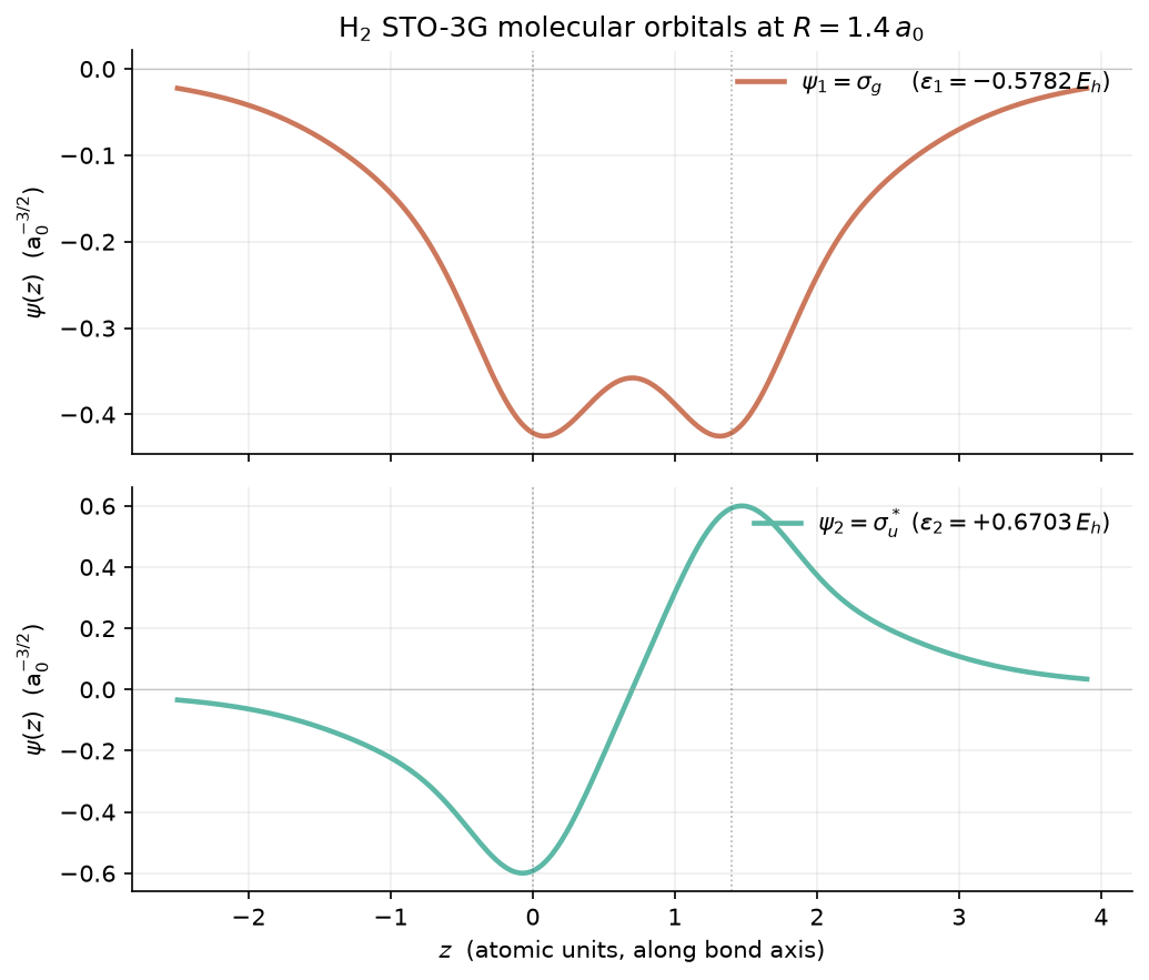
Figure 1. The two molecular orbitals of $\rm H_2$ in the STO-3G basis at $R = 1.4\,a_0$, sampled along the bond axis. Top: $\sigma_g$ bonding orbital ($\varepsilon_1 = -0.578\,E_h$), no node, amplitude concentrated in the bond midpoint. Bottom: $\sigma_u^*$ antibonding orbital ($\varepsilon_2 = +0.670\,E_h$), one node at $z = R/2$, opposite signs on the two atoms.
6.10 The workflow, end to end
%%{init: {'flowchart': {'htmlLabels': true, 'curve': 'basis'}}}%%
graph LR
  M["Molecule or<br/>periodic cell<br/><small>geometry + Z</small>"] --> B{"Choose basis<br/>family"}
  B -->|"atom-centred"| G["Gaussians<br/><small>STO-3G, 6-31G,<br/>cc-pVTZ, aug-cc-pVTZ</small>"]
  B -->|"periodic"| PW["Plane waves<br/><small>E_cut, Brillouin-zone grid</small>"]
  B -->|"finite cluster"| RS["Real-space grid<br/><small>grid spacing h</small>"]
  G --> AO["Build S, h_core,<br/>ERI tensor"]
  PW --> AO2["Build kinetic diagonal,<br/>density on FFT grid"]
  RS --> AO3["Build sparse Laplacian,<br/>diagonal v_xc"]
  AO --> SCF["Roothaan-Hall<br/>FC = SCE<br/><small>iterate to self-consistency</small>"]
  AO2 --> SCF
  AO3 --> SCF
  SCF --> OUT["Orbitals, density,<br/>total energy"]
  OUT --> CHK{"Converged with<br/>basis?"}
  CHK -->|"no"| B
  CHK -->|"yes"| DONE["Report E, ρ, forces"]
The decision in the top-left box is the one a practitioner spends most of their time on. Atom-centred Gaussians dominate finite-molecule chemistry; plane waves dominate solid-state physics; real-space grids are a niche favoured for parallelisation and for systems where the periodicity assumption is awkward. All three feed the same self-consistent loop and, in the basis-set limit, give the same answer.
6.11 Problems
Problem 1 (easy) — Counting basis functions for water
Water (H$_2$O) has one O and two H atoms. Count the number of contracted basis functions $K$ that the basis sets **STO-3G**, **6-31G**, **6-31G***, and **cc-pVDZ** give for water. Use the per-atom compositions stated in sections 6.4–6.6 and the spherical-harmonic convention for $d$-functions (5 per shell, not 6).Show answer
Per-atom contributions: | Basis | H (per atom) | O (per atom) | $K$ for H$_2$O | |:---------|:-------------|:-------------|:------------------| | STO-3G | $1s$ → 1 | $1s, 2s, 2p_{x,y,z}$ → 5 | $1 \cdot 2 + 5 = 7$ | | 6-31G | $1s, 1s'$ → 2 | $1s, 2s, 2s', 2p, 2p'$ → 9 | $2 \cdot 2 + 9 = 13$ | | `6-31G*' | same as 6-31G | + $3d$ (5 spherical) → 14 | $2 \cdot 2 + 14 = 18$ | | cc-pVDZ | $(2s, 1p)$ → 5 | $(3s, 2p, 1d)$ → $3 + 6 + 5 = 14$ | $5 \cdot 2 + 14 = 24$ | (For cc-pVDZ the $1p$ on H is one shell of three Cartesian $p$-functions, i.e. five basis functions per H: two $s$ and three $p$.) The headline numbers: STO-3G gives $K = 7$, 6-31G gives $K = 13$, `6-31G*' gives $K = 18$, cc-pVDZ gives $\boxed{K = 24}$ — and cc-pVTZ, cc-pVQZ, cc-pV5Z grow to 58, 115, 201 respectively. The ERI count scales as $K^4$, so each step up the ladder is a factor of 5–10 more expensive.Problem 2 (medium) — Prove the Gaussian product theorem
Show by direct algebra that for any two centres $\mathbf A, \mathbf B \in \mathbb R^3$ and positive exponents $\alpha, \beta$, $$ e^{-\alpha |\mathbf r - \mathbf A|^2}\, e^{-\beta |\mathbf r - \mathbf B|^2} \;=\; e^{-\alpha\beta/(\alpha+\beta)\, |\mathbf A - \mathbf B|^2}\, e^{-(\alpha+\beta) |\mathbf r - \mathbf P|^2} , $$ where $\mathbf P = (\alpha \mathbf A + \beta \mathbf B)/(\alpha+\beta)$. You may work in one dimension; the three-dimensional result follows from the factorisation $|\mathbf r - \mathbf A|^2 = \sum_{i \in \{x,y,z\}} (r_i - A_i)^2$.Show answer
In one dimension, write the exponent of the product as $$ -\alpha (r - A)^2 - \beta (r - B)^2 \;=\; -(\alpha + \beta) r^2 + 2(\alpha A + \beta B) r - (\alpha A^2 + \beta B^2) . $$ Define $p = \alpha + \beta$ and $P = (\alpha A + \beta B)/p$, so the linear coefficient $2 p P$ matches. Completing the square in $r$, $$ -p r^2 + 2 p P\, r - (\alpha A^2 + \beta B^2) \;=\; -p (r - P)^2 + p P^2 - (\alpha A^2 + \beta B^2) . $$ It remains to evaluate the constant $\;p P^2 - (\alpha A^2 + \beta B^2)\;$. Substituting $P = (\alpha A + \beta B)/p$, $$ p P^2 \;=\; \frac{(\alpha A + \beta B)^2}{p} \;=\; \frac{\alpha^2 A^2 + 2\alpha\beta A B + \beta^2 B^2}{\alpha + \beta} . $$ Subtracting $\alpha A^2 + \beta B^2 = (\alpha A^2 + \beta B^2)(\alpha + \beta)/(\alpha + \beta)$ under a common denominator gives $$ p P^2 - (\alpha A^2 + \beta B^2) \;=\; \frac{\alpha^2 A^2 + 2\alpha\beta A B + \beta^2 B^2 - (\alpha + \beta)(\alpha A^2 + \beta B^2)}{\alpha + \beta} . $$ Expanding the second numerator term, $(\alpha + \beta)(\alpha A^2 + \beta B^2) = \alpha^2 A^2 + \alpha\beta B^2 + \alpha\beta A^2 + \beta^2 B^2$, and cancelling the $\alpha^2 A^2$ and $\beta^2 B^2$ pieces, $$ p P^2 - (\alpha A^2 + \beta B^2) \;=\; \frac{2 \alpha\beta A B - \alpha\beta (A^2 + B^2)}{\alpha + \beta} \;=\; - \frac{\alpha \beta}{\alpha + \beta} (A - B)^2 . $$ Therefore the exponent of the product is $$ -(\alpha + \beta)(r - P)^2 \;-\; \frac{\alpha\beta}{\alpha + \beta}(A - B)^2 , $$ which exponentiates to the claimed identity. In three dimensions, repeat for each Cartesian component; $(A - B)^2$ accumulates to $|\mathbf A - \mathbf B|^2$ and the $(r - P)^2$ piece becomes $|\mathbf r - \mathbf P|^2$. $\quad\blacksquare$Problem 3 (hard) — Plane-wave count and Hamiltonian cost
A cubic simulation cell of side $L = 10\,$Å is used to contain an isolated water molecule. In atomic units, $L = 10 / 0.529177 \approx 18.897\,a_0$, so $\Omega = L^3 \approx 6748\,a_0^3$. Compute: 1. The number of plane waves $N_\text{PW}$ at the $\Gamma$ point ($\mathbf k = \mathbf 0$) for kinetic-energy cutoffs $E_\text{cut} = 30\,E_h$, $60\,E_h$, $100\,E_h$. 2. The corresponding diagonalisation cost ratios (full diagonalisation is $\mathcal O(N_\text{PW}^3)$). 3. Discuss qualitatively why a pseudopotential ([chapter 08](/DFT-notes/dft-notes/chapter-08/)) can reduce $E_\text{cut}$ from $\sim 100\,E_h$ (all-electron for first-row atoms) to $\sim 30$–$50\,E_h$.Show answer
**Step 1.** Apply \eqref{eq:ch-06-npw} directly, $$ N_\text{PW} \;=\; \frac{\Omega}{6 \pi^2}\, (2 E_\text{cut})^{3/2} , \qquad \Omega = 6748\,a_0^3, \quad 6\pi^2 \approx 59.22 . $$ For $E_\text{cut} = 30\,E_h$: $(2 \cdot 30)^{3/2} = 60^{3/2} = \sqrt{60^3} = \sqrt{216000} \approx 464.8$. $\;N_\text{PW} \approx 6748 \cdot 464.8 / 59.22 \approx 52{,}966.$ For $E_\text{cut} = 60\,E_h$: $(2 \cdot 60)^{3/2} = 120^{3/2} \approx 1314.5$. $\;N_\text{PW} \approx 6748 \cdot 1314.5 / 59.22 \approx 149{,}787.$ For $E_\text{cut} = 100\,E_h$: $(2 \cdot 100)^{3/2} = 200^{3/2} \approx 2828.4$. $\;N_\text{PW} \approx 6748 \cdot 2828.4 / 59.22 \approx 322{,}308.$ **Step 2.** Full diagonalisation is $\mathcal O(N_\text{PW}^3)$. Relative costs, normalised to $E_\text{cut} = 30$: | $E_\text{cut}$ | $N_\text{PW}$ | $N_\text{PW}^3$ (relative) | |:---------------|--------------:|---------------------------:| | 30 $E_h$ | 52 966 | 1 | | 60 $E_h$ | 149 787 | $\approx 22.6$ | | 100 $E_h$ | 322 308 | $\approx 225$ | Doubling the cutoff costs a factor of $2^{4.5} \approx 22.6$ (the basis grows as $E_\text{cut}^{3/2}$ and the cubic diagonalisation eats another factor of $E_\text{cut}^{3/2}$ on top), and tripling the cutoff costs more than two orders of magnitude. **Step 3.** An all-electron description of, say, oxygen needs plane waves that resolve the $1s$ orbital, whose characteristic length scale is $\sim 1/Z = 1/8\,a_0$. By the real-space grid argument \eqref{eq:ch-06-grid-cutoff} this requires $E_\text{cut} \gtrsim \pi^2 / (2 \cdot (1/8)^2) \approx 316\,E_h$ — hopeless for a plane-wave code. A pseudopotential replaces the $1s$ (and $2s$) core orbitals by a smooth effective potential whose Fourier components die off above $|\mathbf G| \sim 6$–$8\,a_0^{-1}$, so a cutoff of $30$–$50\,E_h$ is enough. In practice every plane-wave DFT calculation on anything heavier than helium uses a pseudopotential — the quadratic cost saving (from $\sim 225$ down to $1$) is what makes the method usable at all.6.12 What we left out
This chapter scratched the surface of basis-set design. Some of what we skipped:
- Basis-set superposition error (BSSE). When two fragments are computed in the union of their atomic bases, each fragment can use functions centred on the other to artificially lower its own energy. The standard fix is the counterpoise correction (Boys & Bernardi 1970). We ignored it.
- Numerical atom-centred orbitals. Codes like SIESTA, DMol3, and FHI-aims use numerically tabulated atomic orbitals — a third family between Gaussians and plane waves — that are systematically improvable like Gaussians but carry no contraction-fitting error. We did not discuss them.
- Resolution-of-the-identity / density-fitting. The ERI tensor $(ij|kl)$ is the bottleneck of every Gaussian SCF. Density-fitting (DF / RI) approximates it as a product of three-centre integrals over an auxiliary basis, reducing storage from $\mathcal O(K^4)$ to $\mathcal O(K^3)$. Standard in every production code; out of scope here.
- Effective-core potentials (ECPs) and relativistic contractions. For heavy elements ($Z \gtrsim 30$) the inner-shell electrons demand a relativistic treatment and a basis tuned for it. We will revisit this in chapter 08 in the pseudopotential context.
- Wavelets and B-splines. Multiresolution and finite- element methods (BigDFT, FHI-aims’ NAOs) avoid the uniform-grid Nyquist limit and are increasingly relevant for large molecules. We mentioned them in passing only.
Next: chapter 07 — Bloch’s theorem and the Brillouin zone: how plane waves and $k$-points combine to handle infinite periodic solids.
6.13 Numerical atomic orbitals (NAOs)
The basis sets of sections 6.3–6.6 (STO-nG, Pople, Dunning) are all analytic: every function in the basis is known in closed form as a sum of Gaussians. An alternative, used by SIESTA (linear-scaling DFT), FHI-aims (numeric all-electron), and the partial-wave construction of PAW (section 6.15), is to tabulate each basis function numerically on a radial grid. The basis functions are still atom-centred and angular-momentum- resolved, but the radial part is a numerical solution of a one-particle Schrödinger equation — there are no contraction coefficients and no least-squares fitting error. The price is that the integrals are not analytical; they are evaluated by quadrature on the same radial grid the orbital was defined on.
6.13.1 The claim
A numerical atomic orbital (NAO) of angular momentum $\ell$ and “zeta index” $q$ centred at atom $a$ is
\[\label{eq:ch-06-13-nao} \chi_{\ell m}^{(a, q)}(\mathbf r) \;=\; R_\ell^{(a, q)}(r_a)\, Y_{\ell m}(\hat{\mathbf r}_a) , \qquad \mathbf r_a \equiv \mathbf r - \mathbf R_a ,\]where $Y_{\ell m}$ is a real spherical harmonic, $r_a$ is the distance to atom $a$, and the radial function $R_\ell^{(a,q)}$ is a numerical solution of a modified radial Schrödinger equation with a confining potential. The index $q = 1, 2, \dots, n_\zeta$ labels the multiple-ζ split of the valence shell.
6.13.2 The radial Schrödinger equation
The atomic problem for the radial part of an orbital in a spherically symmetric effective potential $V_\text{eff}(r)$ is
\[\label{eq:ch-06-13-radial} \left[ -\frac{1}{2} \frac{d^2}{dr^2} + \frac{\ell(\ell+1)}{2 r^2} + V_\text{eff}(r) \right]\, u_\ell(r) \;=\; \varepsilon\, u_\ell(r) ,\]where $u_\ell(r) = r\, R_\ell(r)$ is the radial function scaled by $r$ (so the volume element $r^2 dr\, d\Omega$ becomes just $du\, d\Omega$). The boundary conditions are
- $u_\ell(0) = 0$ (the wavefunction must vanish at the nucleus),
- $u_\ell(r) \to 0$ as $r \to \infty$ (bound-state decay).
In an isolated atom the second condition is automatically satisfied because $V_\text{eff}$ is attractive. In a molecule, however, the valence NAO must be representable on a finite support, or the overlap matrix becomes ill-conditioned and the SCF converges poorly. The fix is to add a confining potential to $V_\text{eff}$ that vanishes in the chemically relevant region and rises outside it:
\[\label{eq:ch-06-13-confine} \tilde V_\text{eff}(r) \;=\; V_\text{eff}(r) + V_\text{conf}(r) .\]A widely used form (SIESTA, FHI-aims) is a polynomial ramp,
\[\label{eq:ch-06-13-vconf} V_\text{conf}(r) \;=\; \begin{cases} 0 , & r \le r_0 , \\\\[2pt] V_0 \left( \dfrac{r - r_0}{R_c - r_0} \right)^n , & r_0 < r \le R_c , \\\\[6pt] \infty , & r > R_c , \end{cases}\]with the “inner radius” $r_0$ set to roughly the covalent radius of the atom (so the confining potential does not touch the bond region) and the confinement radius $R_c$ the control parameter the user varies. Common choices are $n = 2$ (quadratic) and $V_0 \sim 50$–$100\,E_h$. With this $V_\text{conf}$ the radial equation \eqref{eq:ch-06-13-radial} becomes a bound-state problem in a finite box, solvable by Numerov or by shooting to the asymptotic boundary $r = R_c$ where $u_\ell(R_c) = 0$.
6.13.3 The logarithmic grid
The radial equation is stiff at small $r$ (where $\ell(\ell+1)/2r^2$ diverges and the wavefunction oscillates rapidly) and smooth at large $r$ (where it decays exponentially). A uniform grid wastes resolution in the asymptotic region. The standard choice is the **logarithmic grid introduced by H. J. A. M. Kormann and used in SIESTA and FHI-aims:
\[\label{eq:ch-06-13-loggrid} r_i \;=\; r_\text{min}\, e^{h\, i} , \qquad i = 0, 1, 2, \dots, N_r - 1 .\]The grid has constant log-spacing $h$ — i.e. constant relative resolution. Typical parameters: $r_\text{min} \sim 10^{-4}\,a_0$, $h \sim 0.03$–$0.05\,a_0$, $N_r \sim 500$–$2000$. At the heavy end of the basis (PAW partial waves, see section 6.15) one uses a denser log grid with $h \sim 0.01\,a_0$ and $N_r \sim 2000$ to resolve the oscillations of the $1s$ orbital near the nucleus.
Substituting \eqref{eq:ch-06-13-loggrid} into \eqref{eq:ch-06-13-radial} removes the singular $\ell(\ell+1)/2r^2$ behaviour at small $r$ (because $\ell(\ell+1)/(2 r^2) = \ell(\ell+1)/(2 r_\text{min}^2)\, e^{-2hi}$ is finite at $i=0$ and decays geometrically), and the Numerov method becomes uniformly accurate across the whole grid.
6.13.4 Multiple-ζ
A single NAO per $(\ell, m)$ is a single-ζ basis: it captures the size of the valence orbital but not its flexibility under chemical bonding. The multiple-ζ idea (Artacho, Sánchez-Portal, Ordejón, Soler 1998; Junquera, Paz, Sánchez-Portal, Artacho 2001) is to generate $n_\zeta$ NAOs for the same $(\ell, m)$ by solving the same radial equation with different confinement radii and orthogonalising the higher ζ’s against the lower ones.
Concretely, for a double-ζ valence shell ($n_\zeta = 2$):
- First ζ. Solve \eqref{eq:ch-06-13-radial} with $\tilde V_\text{eff}$ at the “tight” radius $R_c = R_\text{min}$ (typically half the bond length). Call the lowest-lying solution $R_\ell^{(1)}(r)$.
- Second ζ. Solve again with the “loose” radius $R_c = R_\text{max}$ (typically the bond length). Call the new solution $\tilde R_\ell(r)$. Symmetric-orthogonalise against $R_\ell^{(1)}$:
- Higher ζ. Repeat the procedure with progressively looser $R_c$, projecting out the span of all previous ζ’s.
The smaller the inner $\zeta$, the more compact and rigid it is; the larger the outer $\zeta$, the more diffuse and responsive to bonding. This is exactly the chemistry that Pople’s split-valence (6-31G, 6-311G) tried to encode empirically, but now the split-ζ functions are ground-state solutions of the atomic problem rather than ad-hoc contractions. In SIESTA, a typical valence basis is SZ (single-ζ) for production-quality geometry optimisation, DZ (double-ζ) for property prediction, and TZDP (triple-ζ + double polarisation) for high accuracy. The energy cost of an NAO basis is essentially that of a Gaussian basis of the same $K$ — but the information content per function is higher, so a DZ NAO basis often gives an accuracy comparable to a TZ Gaussian basis.
6.13.5 Polarisation orbitals
The multiple-ζ trick handles the radial flexibility. The angular flexibility (which is what polarisation functions do in a Gaussian basis) is generated by an energy-derivative recipe (Blöchl 1990, generalised by Artacho et al.):
\[\label{eq:ch-06-13-pold} R_\ell^\text{pol}(r) \;=\; \mathcal N\, \frac{\partial R_\ell(r)}{\partial \varepsilon} .\]The derivative of a bound-state radial wavefunction with respect to its energy is automatically orthogonal to the parent function $R_\ell$ (the Hellmann–Feynman argument: $\langle R_\ell | \partial R_\ell / \partial \varepsilon \rangle = -\tfrac{1}{2}\, \partial_\varepsilon \langle R_\ell | R_\ell \rangle = 0$ for normalised $R_\ell$). It also has a node — it changes sign once — so it carries the next angular-momentum character after projection. Specifically, if $R_\ell$ is the valence s-function, $\partial_\varepsilon R_\ell$ behaves like a p-function under angular integration; this is the NAO analogue of adding a $p$-polarisation function on hydrogen.
Higher polarisation orbitals — e.g. the “double polarisation” of a TZDP basis — are obtained by a second derivative $\partial^2 R_\ell / \partial \varepsilon^2$, projected against the span of ${\partial_\varepsilon R_\ell}$ and the valence $R_\ell$.
6.13.6 Convergence with $R_c$
The accuracy of an NAO basis depends monotonically on $R_c$: looser confinement (larger $R_c$) makes the basis more flexible and the BSIE smaller, at the cost of a longer-ranged, more-overlapping, and more linearly-dependent basis. In practice SIESTA and FHI-aims report a typical convergence study for the atomisation energy of a small molecule (e.g. $\mathrm H_2 \mathrm O$ or benzene): the energy converges to within $0.01\,E_h$ at $R_c \sim 4\,a_0$ (DZ), $\sim 5\,a_0$ (TZ), $\sim 6\,a_0$ (TZDP). Below $R_c \sim 2.5\,a_0$ the basis is too tight to describe the bonding and the energy becomes wildly wrong.
A more formal diagnostic is the basis-set limit curve $E(K)$ plotted on a log–log axis: for an NAO basis $E(K)$ falls approximately as $K^{-p}$ with $p \sim 2$–$3$ (the exact exponent depends on the confining-potential shape and on the property being converged — total energies converge faster than energy differences).
Note. In PAW (section 6.15) the NAO machinery is re-used for the partial waves $\phi_i^a$ inside the augmentation sphere. The radial grid and the confining potential are the same; only the role changes — there the NAO is an auxiliary object used to reconstruct the AE wavefunction from the smooth part, not a basis function in its own right.
6.13.7 SIESTA workflow
graph LR
  A["Atomic problem:<br/>Z_a + boundary"] --> B["Solve radial<br/>Schrödinger<br/>Numerov on log grid"]
  B --> C1["1st ζ (tight R_c)"]
  B --> C2["2nd ζ (loose R_c)"]
  B --> C3["n-th ζ (projected)"]
  C1 --> ORTH["Gram-Schmidt<br/>orthogonalise"]
  C2 --> ORTH
  C3 --> ORTH
  ORTH --> P["Polarisation:<br/>∂R/∂ε"]
  P --> BASIS["NAO basis<br/>{χ_ℓm^(a,q)}"]
  BASIS --> SCF["SCF with O(N)<br/>or O(N^3) solver"]
The Roothaan–Hall machinery of \eqref{eq:ch-06-roothaan-hall} is unchanged: the matrix elements $\langle \chi_\mu | \hat F | \chi_\nu \rangle$ are evaluated by quadrature on the same radial grid that generated $\chi_\mu$, but otherwise the linear algebra of section 6.1 goes through verbatim.
6.14 Wavelets and B-splines
The plane-wave basis of section 6.7 is systematically improvable: pushing $E_\text{cut}$ to infinity gives the exact answer provided the potential is non-singular — which is not the case for the all-electron problem. The atom-centred Gaussian basis of section 6.3 is also systematically improvable in principle — the cc-pVXZ series is built on this premise — but the convergence is angular: the missing angular momenta show up as slowly-decaying multipole errors in the electron density. Wavelets and B-splines are the basis families that are both atom-like (no periodic boundary condition required) and systematically improvable for the all-electron problem.
6.14.1 B-splines on a finite interval
A B-spline of order $k$ (degree $k - 1$) on a knot sequence $t_0 \le t_1 \le \dots \le t_{N}$ is defined by the Cox–de Boor recursion
\[\label{eq:ch-06-14-bspline} B_{i,1}(x) \;=\; \begin{cases} 1 , & t_i \le x < t_{i+1} , \\\ 0 , & \text{otherwise} , \end{cases}\] \[\label{eq:ch-06-14-coxdeboor} B_{i,k}(x) \;=\; \frac{x - t_i}{t_{i+k-1} - t_i}\, B_{i,k-1}(x) \;+\; \frac{t_{i+k} - x}{t_{i+k} - t_{i+1}}\, B_{i+1,k-1}(x) .\]For a simple uniform knot sequence $t_i = i h$, the B-splines are translated copies of one function $B_k(x/h)$, each supported on $k$ adjacent intervals. The order-$k$ B-spline is a piecewise polynomial of degree $k-1$, $C^{k-2}$ continuous at the interior knots, and identically zero outside its $k$-interval support.
The partition of unity property
\[\label{eq:ch-06-14-pou} \sum_{i=0}^{N-k} B_{i,k}(x) \;=\; 1 \qquad \text{on the interior}\]follows by induction on $k$ and makes B-splines a natural finite-element basis. In 3D the tensor product $B_{i,k}(x)\, B_{j,k}(y)\, B_{\ell,k}(z)$ is a piecewise polynomial of degree $3(k-1)$ on a uniform cubic grid of spacing $h$.
B-splines are the basis of choice in finite-element discretisations of the Kohn–Sham problem (FEM-DFT codes such as HelFEM and parts of FHI-aims in their all-electron NAO mode). They give an exact representation of polynomials up to degree $k-1$, have controllable smoothness (raise $k$ for smoother wavefunctions), and are the finite-dimensional subspace against which the variational principle \eqref{eq:ch-06-variational} is taken. The kinetic-energy operator in a B-spline basis is a banded matrix of bandwidth $\sim k$, so the sparse direct solver scales as $\mathcal O(N_g k^2)$ for a grid of $N_g$ points.
6.14.2 Daubechies wavelets
A wavelet basis is a multiresolution generalisation of the B-spline idea: instead of a single grid, one uses an infinite tower of grids, doubling the resolution at each level. Define a chain of closed subspaces
\[\label{eq:ch-06-14-mra} \\{ 0 \\} \;\subset\; \cdots \;\subset\; V_1 \;\subset\; V_2 \;\subset\; \cdots \;\subset\; L^2(\mathbb R) ,\]with $V_{j+1} = V_j \oplus W_j$ — i.e. the detail space $W_j$ is the orthogonal complement of $V_j$ in $V_{j+1}$. Each $V_j$ is spanned by translations and dyadic scalings of a single scaling function $\phi$:
\[\label{eq:ch-06-14-vj} V_j \;=\; \overline{\text{span}\big\lbrace \phi_{j,k}(x) = 2^{j/2}\, \phi(2^j x - k) : k \in \mathbb Z \big\rbrace} .\]The Daubechies family D-$N$ is parametrised by the number of vanishing moments $N$ and constructed as the most localised orthonormal scaling function with $N$ vanishing moments — the support of the D-$N$ scaling function is $2N - 1$ grid points wide. The two-scale relation between $\phi$ and the orthonormal wavelet $\psi$ is
\[\label{eq:ch-06-14-twoscale} \phi(x) \;=\; \sqrt{2} \sum_{n} h_n\, \phi(2x - n) , \qquad \psi(x) \;=\; \sqrt{2} \sum_{n} g_n\, \phi(2x - n) ,\]where the low-pass filter $h_n$ and high-pass filter $g_n$ are finite sequences of $2N$ coefficients satisfying the quadrature-mirror conditions $g_n = (-1)^n h_{1-n}$ and $\sum_n h_n h_{n + 2k} = \delta_{k,0}$. For D-2 the filters are
\[h_0 = \tfrac{1 + \sqrt 3}{4 \sqrt 2}, \quad h_1 = \tfrac{3 + \sqrt 3}{4 \sqrt 2}, \quad h_2 = \tfrac{3 - \sqrt 3}{4 \sqrt 2}, \quad h_3 = \tfrac{1 - \sqrt 3}{4 \sqrt 2},\]and the scaling function has support $[0, 3]$. Higher $N$ gives smoother $\phi$ and $\psi$ (the D-$N$ scaling function is $C^{\alpha N}$ for some $\alpha < 1$) at the cost of longer filters.
6.14.3 Why wavelets are systematically improvable
The B-spline basis of section 6.14.1 is complete in the sense that the finite-element space $V_J$ becomes dense in $L^2$ as $J \to \infty$ (i.e. as the grid spacing $h \to 0$). The wavelet basis of section 6.14.2 is complete for the same reason — $V_J$ is spanned by translated B-spline-like scaling functions. The additional thing the wavelet basis gives is adaptivity: a function with sharp features (near a nucleus, say) is represented economically in $V_J$ because the wavelet coefficients on the coarse level $W_{J - 1}$ capture the high-frequency content that would otherwise force a uniform refinement to a much finer grid.
For the all-electron problem, this adaptivity is essential. The $1s$ wavefunction of a carbon atom oscillates on a lengthscale of $\sim 0.1\,a_0$ near the nucleus, but is smooth and slowly-varying at the bond radius $\sim 1.5\,a_0$. A uniform grid that resolves the $1s$ oscillation at $h \sim 0.05\,a_0$ would need $\sim 10^7$ grid points in a $10\,a_0$ cell — wasted on the chemically relevant valence region. A wavelet basis on the same domain (BigDFT uses D-2 to D-8 wavelets) reaches the same accuracy with $\sim 10^5$ coefficients, because the wavelet coefficients in the valence region are sparse.
This is the formal claim:
\[\label{eq:ch-06-14-wavelet-conv} E_\text{total}(J) \;=\; E_\text{exact} \;+\; \mathcal O(2^{-s J}) , \qquad s \ge 1\]for $J$ wavelet levels — exponential convergence in the number of levels, and the only basis family for which this claim holds with the full all-electron Coulomb singularity (no pseudopotential, no PAW).
6.14.4 The BigDFT code
The BigDFT code (Genovese et al. 2008; Mohr et al. 2014) implements Kohn–Sham DFT in a Daubechies-wavelet basis on a cubic simulation cell with two grids: a coarse grid for the density and Hartree potential, and a fine grid (eight times finer) for the orbitals. The two-grid treatment of the non-local exchange term — the most expensive part of hybrid DFT — gives BigDFT its best-in-class scaling with system size for non-periodic systems: $\mathcal O(N)$ for the total energy (when the locality of the density matrix is exploited) and $\mathcal O(N \log N)$ for the diagonalisation step.
graph LR
  R["Cubic cell<br/>(0, L)^3"] --> M["Multi-resolution<br/>analysis"]
  M --> C["Coarse grid<br/>(density, v_H)"]
  M --> F["Fine grid<br/>(orbitals)"]
  C --> POIS["Multigrid Poisson<br/>solver (FFT-free)"]
  F --> KS["Kohn-Sham<br/>sparse matrix"]
  POIS --> KS
  KS --> E["Total energy,<br/>forces"]
The Mermaid diagram shows the structure: the wavelet basis provides both grids simultaneously from the same multi-resolution analysis, and the Poisson solver is exact in the wavelet basis (no FFT, no periodic boundary condition required, no vacuum buffer for finite molecules).
Note. Wavelets are orthogonal, so $\mathbf S = \mathbf I$ and the Roothaan–Hall equation \eqref{eq:ch-06-roothaan-hall} collapses to the standard eigenproblem $\mathbf F \mathbf C = \mathbf C \boldsymbol\varepsilon$. This is the first basis in this chapter where the overlap matrix is automatically trivial.
6.15 Plane-wave projector augmented waves (PAW)
The plane-wave basis of section 6.7 is the basis of periodic solids, but it cannot resolve the all-electron Coulomb singularity at the nucleus. A pseudopotential (chapter 08) replaces the singularity by a smooth effective potential — at the price of giving up all information about the wavefunction near the nucleus. Projector augmented waves (PAW; Blöchl 1994; Kresse & Joubert 1999) keep the plane-wave basis for the “easy” region between the atoms, but augment it with an exact atomic solution inside a small sphere around each atom. PAW is the method used in VASP, Quantum ESPRESSO, GPAW, Castep, CP2K (in the GPW mode), and ABINIT; we will meet the pseudopotential limit of it in chapter 08.
6.15.1 The PAW transformation
Let $\phi_i^a(\mathbf r)$ be the all-electron (AE) partial wave of atom $a$, with composite index $i = (n, \ell, m)$ standing for the principal, angular, and magnetic quantum numbers of the AE solution inside the augmentation sphere. Let $\tilde\phi_i^a(\mathbf r)$ be the corresponding pseudo partial wave — the smooth function that equals $\phi_i^a$ outside the augmentation sphere of radius $r_c^a$ and is regular at the nucleus. The projector $\tilde p_i^a$ is the dual of $\tilde\phi_i^a$,
\[\label{eq:ch-06-15-dual} \langle \tilde p_i^a \mid \tilde\phi_j^b \rangle \;=\; \delta_{ab}\, \delta_{ij} ,\]where the integral is over the augmentation sphere of atom $a$ only. The PAW transformation is
\[\label{eq:ch-06-15-trafo} \hat{\mathcal T} \;=\; \hat 1 \;+\; \sum_a \sum_i \left( \lvert \phi_i^a \rangle - \lvert \tilde\phi_i^a \rangle \right) \langle \tilde p_i^a \rvert .\]Applied to a smooth wavefunction $\lvert \tilde \psi_n \rangle$ it produces the AE wavefunction
\[\label{eq:ch-06-15-reconstruct} \lvert \psi_n \rangle \;=\; \hat{\mathcal T} \lvert \tilde \psi_n \rangle \;=\; \lvert \tilde \psi_n \rangle \;+\; \sum_{a,i} \left( \lvert \phi_i^a \rangle - \lvert \tilde\phi_i^a \rangle \right) \langle \tilde p_i^a \rvert \tilde \psi_n \rangle .\]The right-hand side is the PAW reconstruction: the smooth wavefunction $\tilde\psi_n$ plus a sum over atoms and partial-wave indices of the mismatch $\phi_i^a - \tilde\phi_i^a$, weighted by the projection of $\tilde\psi_n$ onto the corresponding projector. Outside the augmentation spheres $\phi_i^a = \tilde\phi_i^a$ by construction, so the correction vanishes; inside each sphere, $\tilde\psi_n$ is replaced by the exact AE expansion in the partial-wave basis.
6.15.2 The plane-wave basis applies to $\tilde \psi_n$
The whole point of the PAW construction is that the smooth wavefunction $\tilde \psi_n$ is the object that lives in the plane-wave basis, exactly as in section 6.7:
\[\label{eq:ch-06-15-pw} \tilde \psi_{n,\mathbf k}(\mathbf r) \;=\; \frac{1}{\sqrt \Omega} \sum_{\mathbf G} c_{n,\mathbf k,\mathbf G}\, e^{i (\mathbf k + \mathbf G) \cdot \mathbf r} .\]The plane-wave cutoff $E_\text{cut}$ now has to resolve the pseudo partial waves $\tilde\phi_i^a$, not the AE $\phi_i^a$. Because $\tilde\phi_i^a$ is smooth at the nucleus, the typical $E_\text{cut}$ drops from $\sim 1000\,E_h$ (all-electron) to $\sim 30$–$80\,E_h$ (PAW with a $1s$–$3d$ valence). The cost saving is roughly two orders of magnitude in plane-wave count, and two more in the diagonalisation cost — see Problem 3 of section 6.11. ### 6.15.3 Augmentation charges
The PAW density and Kohn–Sham potential are not just evaluated on the plane-wave grid. A separate augmentation treatment is needed inside each sphere. The total electron density is
\[\label{eq:ch-06-15-density} \rho(\mathbf r) \;=\; \tilde \rho(\mathbf r) \;+\; \sum_a \left[ \rho^a(\mathbf r) - \tilde \rho^a(\mathbf r) \right] ,\]where
- $\tilde \rho = \sum_n f_n \lvert \tilde \psi_n \rvert^2$ is the smooth density, defined on the plane-wave grid,
- $\rho^a = \sum_{i,j} D_{ij}^a\, \phi_i^a (\phi_j^a)^*$ is the AE augmentation density, defined on the radial grid of atom $a$,
- $\tilde \rho^a = \sum_{i,j} D_{ij}^a\, \tilde\phi_i^a (\tilde\phi_j^a)^*$ is the PS augmentation density, defined on the same radial grid,
- $D_{ij}^a = \sum_n f_n \langle \tilde p_i^a \mid \tilde \psi_n \rangle \langle \tilde \psi_n \mid \tilde p_j^a \rangle$ is the augmentation density matrix for atom $a$.
The smooth density $\tilde \rho$ contains a small but non-negligible contribution from the augmentation region — $\tilde\phi_i^a (\tilde\phi_j^a)^$ evaluated in $\tilde\rho^a$ is the smooth part, while $\phi_i^a (\phi_j^a)^$ in $\rho^a$ is the AE part. The difference $\rho^a - \tilde\rho^a$ in \eqref{eq:ch-06-15-density} subtracts the smooth part and adds back the AE part, exactly restoring the all-electron density inside the augmentation spheres.
The same split is applied to the local part of the potential and to the Hartree and exchange–correlation contributions. In practical codes the compensation (or “augmentation”) charges $\hat n^a(\mathbf r)$ are added to the smooth density so that the multipole moments of the augmentation charge density $\rho^a - \tilde\rho^a$ are absorbed into the plane-wave Hartree solver. The total potential becomes
\[\label{eq:ch-06-15-potential} V(\mathbf r) \;=\; \tilde V(\mathbf r) \;+\; \sum_a \left[ V^a(\mathbf r) - \tilde V^a(\mathbf r) \right] ,\]with $V^a$ and $\tilde V^a$ tabulated on the radial grid of each atom, and $\tilde V$ a plane-wave-expandable smooth potential.
6.15.4 The frozen-core approximation
The partial-wave basis ${\phi_i^a, \tilde\phi_i^a}$ is local to each atom. The standard choice is to include only the valence in the active set — i.e. to freeze the core orbitals (1s for first-row atoms, 1s2s2p for transition metals, etc.) at the values they have in the isolated atom. In this frozen-core approximation,
\[\label{eq:ch-06-15-frozen} D_{ij}^a \;=\; D_{ij}^{a,\,\text{val}} \;+\; D_{ij}^{a,\,\text{core}} , \qquad D_{ij}^{a,\,\text{core}} \;\text{fixed at the atomic value} .\]The frozen-core term is a one-time constant contribution to the augmentation density matrix of each atom; the SCF procedure never varies it. This is the PAW analogue of the frozen-core approximation in pseudopotential methods (chapter 08), with the crucial difference that the PAW reconstruction \eqref{eq:ch-06-15-reconstruct} can still recover the exact AE value of any frozen-core orbital in post-processing (e.g. the X-ray absorption near-edge structure, XANES), because the partial-wave expansion of the core is still available — the all-electron wavefunction is reconstructed, the core just is not allowed to relax in the SCF.
In PAW with a frozen core the “all-electron” reconstruction \eqref{eq:ch-06-15-reconstruct} becomes
\[\label{eq:ch-06-15-frozen-recon} \lvert \psi_n \rangle \;=\; \lvert \tilde \psi_n \rangle \;+\; \sum_{a,i \in \text{val}} \left( \lvert \phi_i^a \rangle - \lvert \tilde\phi_i^a \rangle \right) \langle \tilde p_i^a \rvert \tilde \psi_n \rangle \;+\; \sum_{a, i \in \text{core}} \lvert \phi_i^a \rangle \langle \tilde p_i^a \rvert \tilde \psi_0^a \rangle ,\]where $\tilde \psi_0^a$ is the smooth part of the atomic core wavefunction. The core term is a constant, atom-centred contribution that depends on the atom type but not on the chemical environment — its only role is to keep the all-electron density correct in the core region.
6.15.5 Workflow
graph LR
  AE["AE problem<br/>(divergent at nucleus)"] -->|"PAW transform"| T["Smooth problem<br/>T|ψ̃⟩ = ε|ψ̃⟩"]
  T -->|"plane-wave basis<br/>(E_cut)"| PW["FFT diagonalisation<br/>on the BZ grid"]
  PW --> RECON["PAW reconstruction<br/>|ψ⟩ = |ψ̃⟩ + (|φ⟩ - |φ̃⟩)⟨p̃|ψ̃⟩"]
  RECON --> OUT["AE ψ, ρ, E"]
The Mermaid diagram shows the data flow. The smooth problem is what the plane-wave code actually solves; the AE observables are reconstructed at the end. The augmentation sphere radius $r_c^a$ is the control parameter — it must be small enough that the augmentation spheres of neighbouring atoms do not overlap (a non-overlap requirement that PAW shares with the LAPW method), but large enough that the partial-wave expansion converges quickly. Typical values are $r_c^a \sim 1.0$–$1.5\,a_0$ for first-row atoms and $\sim 1.5$–$2.0\,a_0$ for transition metals.
6.15.6 What the plane-wave code actually does
A practical PAW calculation (VASP, Quantum ESPRESSO) runs the following inner loop:
- Initial guess. Atomic superposition of the $\tilde\phi_i^a$ partial waves for each atom in the cell.
- Build smooth density. Accumulate $\tilde \rho$ on the FFT grid (cutoff $4 E_\text{cut}$).
- Build smooth potential. Hartree via FFT-based Poisson solver, XC on the grid, ionic on the grid.
- Subtract augmentation charges. Replace the smooth augmentation density $\tilde \rho^a$ on each radial grid by the AE $\rho^a$, and update the local potential accordingly.
- Diagonalise. Standard plane-wave Roothaan–Hall with the non-local projector-augmented-wave Hamiltonian operator $\hat H_\text{PAW}$. Iterative diagonalisation (Davidson, RMM-DIIS, or block-Davidson) keeps the cost tractable.
- Update $D_{ij}^a$. Using the new $\tilde \psi_n$.
- Loop 2–6 to self-consistency.
The “frozen” part of $D_{ij}^a$ (the core) is set in step 1 and never updated.
Tip. The PAW datasets distributed with VASP / Quantum ESPRESSO are not just pseudopotentials — they contain the partial waves and the projectors. Treating them as “potentials” and ignoring the reconstruction is a common source of confusion. The data file you load into a PAW code is a small, atom-type-specific data set ($\sim 10$–$50$ radial functions per atom type) that defines the augmentation sphere, the partial waves, and the projectors.
6.16 What we left out (updated)
The original “what we left out” in section 6.12 still applies, but the three new sections 6.13–6.15 bring their own omissions:
- Linear-scaling NAO. SIESTA’s $\mathcal O(N)$ mode exploits the sparsity of the density matrix in an atom-centred basis; we have not derived the divide-and- conquer or Fermi-operator expansion methods that make this work. See chapter 10 for the linear-scaling toolkit.
- Adaptive finite elements. FEniCS-based DFT codes use unstructured tetrahedral meshes with adaptive refinement, a generalisation of the B-spline idea; we touched on it only in passing.
- LAPW / APW+lo. The linearised augmented plane wave basis (used by FLEUR, Wien2k) is a different augmentation of the plane-wave basis, with energy-linearised partial waves at fixed energy $\varepsilon_\ell$ and “local orbitals” for energy flexibility. PAW is formally equivalent in the limit of large partial-wave sets, but the implementation is different and worth comparing. We did not.
- The ultrasoft pseudopotential limit of PAW. In the limit that the augmentation sphere shrinks to zero and the partial-wave set collapses to a single function, the PAW transformation reduces to an ultrasoft pseudopotential (Vanderbilt 1990) — a connection worked out in chapter 08.
- Wavelet basis sets for molecules. The $\mathcal O(N)$ wavelet DFT codes (BigDFT, ORCHID) combine the wavelet basis with density-matrix purification; we did not derive the purification step.
- Spin–orbit coupling in the PAW augmentation. For heavy elements ($Z \gtrsim 30$) the PAW partial waves must be computed in a relativistic framework (the Dirac equation rather than the Schrödinger equation), and the augmentation charges contain a $j$-dependent contribution. We used the scalar-relativistic approximation throughout.