Chapter 07 — Solids & periodic boundary conditions
A perfect crystal has a Hamiltonian that commutes with every translation by a lattice vector. The eigenfunctions are plane waves modulated by a cell-periodic function — and that single fact is the reason solid-state physics has its own language.
Up to chapter 06 we have been talking about finite systems: atoms and molecules in a box. A real solid is not a finite system. It is an infinite, perfectly periodic array of nuclei, and the electron moves through this array forever. The Schrödinger equation we have to solve is therefore not the molecular one of chapter 01, nor the molecular orbital problem of chapter 04 — it is the same Schrödinger equation, but on a Hamiltonian that has the discrete translational symmetry of the crystal. This chapter is about the consequence of that symmetry: the eigenfunctions factorise into a plane wave and a cell-periodic piece, the energy levels become continuous bands parametrised by a crystal momentum k that lives in a small region of reciprocal space, and the practical calculation collapses from an infinite matrix to a finite matrix indexed by a small set of k-points and a small set of plane waves. The machinery that does this is what every production solid-state code (VASP, Quantum ESPRESSO, CASTEP, ABINIT, …) is built on.
Reading note. This chapter assumes you have read chapters 01–05. It previews material that is covered in detail in chapter 06 (basis sets), chapter 08 (pseudopotentials), chapter 10 (phonons), and chapter 11 (band structures).
7.1 The claim
Bloch’s theorem. Let the Hamiltonian $\hat H$ have the discrete translational symmetry of a Bravais lattice ${\mathbf R}$, \(\begin{equation} \label{eq:ch-07-bloch-translation} \hat H(\mathbf r + \mathbf R) = \hat H(\mathbf r) \quad \text{for every } \mathbf R \in \{\mathbf R\}. \end{equation}\) Then every eigenfunction of $\hat H$ can be written in the form \(\begin{equation} \label{eq:ch-07-bloch} \boxed{\psi_{n\mathbf k}(\mathbf r) = e^{i \mathbf k \cdot \mathbf r}\, u_{n\mathbf k}(\mathbf r),} \end{equation}\) where $\mathbf k$ is a real vector, the band index $n$ labels the eigenstates at a given $\mathbf k$, and the cell-periodic function $u_{n\mathbf k}$ has the same periodicity as the lattice, \(\begin{equation} \label{eq:ch-07-bloch-periodic} u_{n\mathbf k}(\mathbf r + \mathbf R) = u_{n\mathbf k}(\mathbf r) \quad \text{for every } \mathbf R. \end{equation}\)
Equation \eqref{eq:ch-07-bloch} is the single most-quoted line in solid-state physics. It says that every eigenstate of a periodic Hamiltonian is a plane wave $e^{i\mathbf k \cdot \mathbf r}$ multiplied by a function $u_{n\mathbf k}(\mathbf r)$ that knows only about one unit cell. The price is that the quantum number is no longer a single integer $n$ — it is now a continuous vector $\mathbf k$ and a band index $n$.
Tip. The phase factor $e^{i\mathbf k \cdot \mathbf r}$ is sometimes called the Bloch factor, and $u_{n\mathbf k}$ the Bloch function or periodic part of the Bloch wave.
7.2 From finite cluster to infinite solid
A real solid is infinite, but we cannot solve an infinite problem on a finite computer. The standard move is to replace “infinite” by “periodic on a supercell”.
7.2.1 Born–von Karman boundary conditions
Pick three primitive lattice vectors $\mathbf a_1, \mathbf a_2, \mathbf a_3$ and form a supercell of $N_1 \times N_2 \times N_3$ primitive cells. Impose Born–von Karman (BvK) periodic boundary conditions on the supercell: for any wavefunction $\psi$,
\[\label{eq:ch-07-bvk} \psi(\mathbf r + N_i \mathbf a_i) = \psi(\mathbf r), \qquad i = 1, 2, 3.\]The supercell is the basic repeat unit; anything that happens in it is copied $N_1 N_2 N_3$ times to fill space. As $N_1, N_2, N_3 \to \infty$ the BvK cell fills all of $\mathbb R^3$ and we recover the infinite solid.
The boundary conditions \eqref{eq:ch-07-bvk} restrict the allowed wavefunctions. In particular, a plane wave $e^{i\mathbf k \cdot \mathbf r}$ satisfies \eqref{eq:ch-07-bvk} iff
\[\label{eq:ch-07-bvk-k} e^{i \mathbf k \cdot (N_i \mathbf a_i)} = 1 \quad \text{for } i = 1, 2, 3 \;\;\Longrightarrow\;\; \mathbf k \cdot \mathbf a_i = \frac{2\pi m_i}{N_i}, \quad m_i \in \mathbb Z.\]The allowed $\mathbf k$ values are therefore a discrete mesh inside the Brillouin zone (defined in §7.4), with $N_1 N_2 N_3$ points in total — one per primitive cell of the BvK supercell.
7.2.2 From $N$ atoms to $N_\mathbf k$ k-points
The two limits to keep in mind:
| Limit | $N_\text{atoms}$ | $N_\mathbf k$ | What we compute |
|---|---|---|---|
| Molecule | Finite (10–1000) | 1 (the $\Gamma$ point) | Total energy, spectrum |
| Solid (BvK) | $\to \infty$ | $N_1 N_2 N_3$ per BZ | Total energy per cell, bands |
For a molecule, “summing over all states” is the discrete sum $\sum_n$ of chapter 04. For a solid under BvK, every “sum over states” becomes a sum over bands and k-points,
\[\label{eq:ch-07-bvk-sum} \sum_n f(\varepsilon_n) \;\;\longrightarrow\;\; \sum_n \sum_{\mathbf k \in \text{BZ}_\text{mesh}} w_\mathbf k \, f(\varepsilon_{n\mathbf k}),\]with weights $w_\mathbf k = 1 / N_\mathbf k$ (uniform mesh). The mesh has to be fine enough that this sum approximates the BZ integral $\int_\text{BZ} f(\varepsilon_{n\mathbf k}) d\mathbf k$ to the desired accuracy.
Tip. The BvK trick is not a physical boundary condition. It is a mathematical device that makes the infinite problem look finite. The answers it produces are the bulk properties of the infinite solid in the limit $N_1, N_2, N_3 \to \infty$. For a truly periodic system, the device is exact. For a finite cluster, BvK artificially glues opposite faces of the cluster together, which is why it is a bad boundary condition for molecules.
7.3 Derivation of Bloch’s theorem
We prove \eqref{eq:ch-07-bloch} in seven explicit steps. Every step appears below — no “it can be shown that” hand-waves .
Step 1. Define the translation operator
For every Bravais-lattice vector $\mathbf R$, define the operator
\[\label{eq:ch-07-trans-op} (\hat T_{\mathbf R} f)(\mathbf r) := f(\mathbf r + \mathbf R).\]$\hat T_{\mathbf R}$ shifts the argument of a function by $\mathbf R$. It is linear and bounded.
Step 2. $\hat T_{\mathbf R}$ is unitary
For any two square-integrable functions $f, g$:
\[\begin{align} \langle \hat T_{\mathbf R} f \mid \hat T_{\mathbf R} g \rangle &= \int_{\mathbb R^3} \Bigl[(\hat T_{\mathbf R} f)(\mathbf r)\Bigr]^* \, (\hat T_{\mathbf R} g)(\mathbf r) \, d^3r \nonumber \\\ &= \int_{\mathbb R^3} f^*(\mathbf r + \mathbf R) \, g(\mathbf r + \mathbf R) \, d^3r \nonumber \\\ &= \int_{\mathbb R^3} f^*(\mathbf u) \, g(\mathbf u) \, d^3u \quad \text{(substituting } \mathbf u = \mathbf r + \mathbf R,\; d^3u = d^3r) \nonumber \\\ &= \langle f \mid g \rangle. \end{align}\]So $\hat T_{\mathbf R}$ preserves inner products. In particular it preserves norms ($|\hat T_{\mathbf R} f| = |f|$), so it is unitary:
\[\label{eq:ch-07-trans-unitary} \hat T_{\mathbf R}^\dagger = \hat T_{\mathbf R}^{-1}, \qquad \hat T_{\mathbf R}^\dagger = \hat T_{-\mathbf R}.\]Step 3. $\hat T_{\mathbf R}$ commutes with $\hat H$
Compute $\hat T_{\mathbf R} \hat H f$ for an arbitrary smooth $f$. The Hamiltonian in the Born–Oppenheimer picture (chapter 01) is
\[\label{eq:ch-07-hamiltonian} \hat H = -\frac{1}{2} \nabla^2 + V(\mathbf r),\]where $V(\mathbf r)$ is the total (ionic + Hartree + xc) one-electron potential. By the crystal periodicity \eqref{eq:ch-07-bloch-translation}, $V(\mathbf r + \mathbf R) = V(\mathbf r)$ for every $\mathbf R$.
Apply the two operators in succession:
\[\begin{align} \Bigl(\hat T_{\mathbf R} \hat H f\Bigr)(\mathbf r) &= (\hat H f)(\mathbf r + \mathbf R) \nonumber \\\ &= -\tfrac{1}{2} \nabla^2 f(\mathbf r + \mathbf R) + V(\mathbf r + \mathbf R) f(\mathbf r + \mathbf R) \nonumber \\\ &= -\tfrac{1}{2} \nabla^2 f(\mathbf r + \mathbf R) + V(\mathbf r) f(\mathbf r + \mathbf R). \end{align}\]The gradient $\nabla$ in the last line is taken with respect to $\mathbf r$; substituting $\mathbf u = \mathbf r + \mathbf R$ leaves $\nabla_\mathbf r f(\mathbf r + \mathbf R) = \nabla_\mathbf u f(\mathbf u)$, so
\[\label{eq:ch-07-commute} \Bigl(\hat T_{\mathbf R} \hat H f\Bigr)(\mathbf r) = -\tfrac{1}{2} \nabla^2 f(\mathbf r + \mathbf R) + V(\mathbf r) f(\mathbf r + \mathbf R) = \Bigl(\hat H \, \hat T_{\mathbf R} f\Bigr)(\mathbf r).\]The two operators therefore commute:
\[\label{eq:ch-07-commute-final} \boxed{[\hat T_{\mathbf R}, \hat H] = 0 \quad \text{for every } \mathbf R.}\]Step 4. $\hat T_{\mathbf R}$ and $\hat H$ can be simultaneously diagonalised
Two commuting self-adjoint operators on a Hilbert space can be brought to a common diagonal form. (Standard result; the operators have a joint spectral measure.) So there exists a complete orthonormal basis of states that are eigenstates of both $\hat T_{\mathbf R}$ and $\hat H$ simultaneously. We will call these basis states $\psi$.
Step 5. The eigenvalues of $\hat T_{\mathbf R}$ are phase factors
The group of Bravais translations is abelian: $\hat T_{\mathbf R} \hat T_{\mathbf R’} = \hat T_{\mathbf R’} \hat T_{\mathbf R} = \hat T_{\mathbf R + \mathbf R’}$. The eigenvalues of a unitary representation of an abelian group are one-dimensional, i.e. complex numbers of unit modulus. We therefore write
\[\label{eq:ch-07-trans-eigval} \hat T_{\mathbf R} \psi = \lambda(\mathbf R) \, \psi, \qquad |\lambda(\mathbf R)| = 1.\]The map $\mathbf R \mapsto \lambda(\mathbf R)$ is a group homomorphism $\mathbb Z^3 \to U(1)$:
\[\label{eq:ch-07-trans-hom} \lambda(\mathbf R + \mathbf R') = \lambda(\mathbf R) \, \lambda(\mathbf R').\]The most general such homomorphism is $\lambda(\mathbf R) = e^{i \mathbf k \cdot \mathbf R}$ for some fixed vector $\mathbf k \in \mathbb R^3$ (think of $\mathbf k$ as the “Fourier transform” of the homomorphism, with the constraint $e^{i\mathbf k \cdot \mathbf R} = 1$ for every lattice $\mathbf R$ fixing $\mathbf k$ only up to reciprocal-lattice additions).
So the eigenstates of $\hat T_{\mathbf R}$ satisfy
\[\label{eq:ch-07-bloch-phase} \psi(\mathbf r + \mathbf R) = e^{i \mathbf k \cdot \mathbf R} \, \psi(\mathbf r) \quad \text{for every } \mathbf R.\]This is sometimes called the Bloch condition.
Step 6. Define the cell-periodic function $u_{\mathbf k}$
Define
\[\label{eq:ch-07-define-u} u_{\mathbf k}(\mathbf r) := e^{-i \mathbf k \cdot \mathbf r} \, \psi(\mathbf r).\]Equation \eqref{eq:ch-07-bloch} is just a rearrangement of \eqref{eq:ch-07-define-u}; the work is to show that $u_{\mathbf k}$ inherits the lattice periodicity.
Compute $u_{\mathbf k}$ at a translated point:
\[\begin{align} u_{\mathbf k}(\mathbf r + \mathbf R) &= e^{-i \mathbf k \cdot (\mathbf r + \mathbf R)} \, \psi(\mathbf r + \mathbf R) \nonumber \\\ &= e^{-i \mathbf k \cdot \mathbf r} \, e^{-i \mathbf k \cdot \mathbf R} \, \Bigl( e^{i \mathbf k \cdot \mathbf R} \, \psi(\mathbf r) \Bigr) \quad \text{by \eqref{eq:ch-07-bloch-phase}} \nonumber \\\ &= e^{-i \mathbf k \cdot \mathbf r} \, \psi(\mathbf r) \nonumber \\\ &= u_{\mathbf k}(\mathbf r). \end{align}\]The two phase factors cancel exactly, and we have
\[\label{eq:ch-07-u-periodic} u_{\mathbf k}(\mathbf r + \mathbf R) = u_{\mathbf k}(\mathbf r) \quad \text{for every } \mathbf R.\]This is \eqref{eq:ch-07-bloch-periodic}, and it completes the proof: the eigenfunction factorises as $\psi(\mathbf r) = e^{i \mathbf k \cdot \mathbf r} u_{\mathbf k}(\mathbf r)$ with $u_{\mathbf k}$ cell- periodic. $\blacksquare$
Note. The crystal momentum $\mathbf k$ is defined only modulo a reciprocal-lattice vector: if $\mathbf G$ is a reciprocal-lattice vector, then $e^{i \mathbf G \cdot \mathbf R} = 1$ for every direct lattice $\mathbf R$, so $\mathbf k$ and $\mathbf k + \mathbf G$ satisfy the same Bloch condition \eqref{eq:ch-07-bloch-phase}. The unique representative of $\mathbf k$ is therefore chosen inside the first Brillouin zone.
7.4 The Brillouin zone
7.4.1 The reciprocal lattice
The set of vectors ${\mathbf G}$ for which $e^{i \mathbf G \cdot \mathbf R} = 1$ for every direct-lattice vector $\mathbf R$ is itself a Bravais lattice, the reciprocal lattice. If the direct lattice has primitive vectors $\mathbf a_1, \mathbf a_2, \mathbf a_3$, the reciprocal lattice has primitive vectors $\mathbf b_1, \mathbf b_2, \mathbf b_3$ defined by
\[\label{eq:ch-07-reciprocal-def} \mathbf a_i \cdot \mathbf b_j = 2\pi \delta_{ij}.\]An explicit construction is
\[\label{eq:ch-07-reciprocal-explicit} \mathbf b_1 = \frac{2\pi \, \mathbf a_2 \times \mathbf a_3}{\mathbf a_1 \cdot (\mathbf a_2 \times \mathbf a_3)}, \qquad \text{and cyclic permutations}.\]Every reciprocal-lattice vector is an integer combination $\mathbf G = h \mathbf b_1 + k \mathbf b_2 + l \mathbf b_3$ with $h, k, l \in \mathbb Z$. The volume of the reciprocal primitive cell is
\[\label{eq:ch-07-reciprocal-volume} V_\text{BZ}^* = \mathbf b_1 \cdot (\mathbf b_2 \times \mathbf b_3) = \frac{(2\pi)^3}{V_\text{cell}},\]where $V_\text{cell} = \mathbf a_1 \cdot (\mathbf a_2 \times \mathbf a_3)$ is the direct-lattice primitive-cell volume.
7.4.2 The first Brillouin zone
The first Brillouin zone (1st BZ) is the Wigner–Seitz cell of the reciprocal lattice: the set of points in reciprocal space that are closer to the origin than to any other reciprocal-lattice point. Its boundary is built from the perpendicular bisector planes of the shortest $\mathbf G$ vectors. Formally,
\[\label{eq:ch-07-bz} \text{1st BZ} = \left\lbrace \mathbf k \in \mathbb R^3 \;:\; |\mathbf k| \le |\mathbf k - \mathbf G| \text{ for every reciprocal-lattice vector } \mathbf G \right\rbrace.\]Every physically distinct crystal momentum is represented exactly once in the 1st BZ, so the “sum over $\mathbf k$” in \eqref{eq:ch-07-bvk-sum} runs over the 1st BZ.
7.4.3 High-symmetry points for the FCC lattice
As an example, the reciprocal lattice of a face-centred cubic (FCC) direct lattice is body-centred cubic (BCC). The primitive vectors of the FCC lattice with conventional cubic parameter $a$ are
\[\label{eq:ch-07-fcc-primitive} \mathbf a_1 = \frac{a}{2}(0, 1, 1),\quad \mathbf a_2 = \frac{a}{2}(1, 0, 1),\quad \mathbf a_3 = \frac{a}{2}(1, 1, 0).\]Equation \eqref{eq:ch-07-reciprocal-explicit} gives the reciprocal primitive vectors
\[\label{eq:ch-07-fcc-reciprocal} \mathbf b_1 = \frac{2\pi}{a}(-1, 1, 1),\quad \mathbf b_2 = \frac{2\pi}{a}(1, -1, 1),\quad \mathbf b_3 = \frac{2\pi}{a}(1, 1, -1),\]which span a BCC lattice. The shortest $\mathbf G$ vectors are $\pm \tfrac{2\pi}{a}(1,1,1)$ and permutations with sign, with length $\tfrac{2\pi}{a}\sqrt{3}$. The 1st BZ of FCC is therefore a truncated octahedron, bounded by:
- 6 square faces at $\pm \tfrac{2\pi}{a}(1,0,0)$ and permutations (perpendicular bisectors of $\mathbf G = \tfrac{4\pi}{a}(\pm 1, 0, 0)$ and permutations);
- 8 hexagonal faces at $\pm \tfrac{\pi}{a}(1, 1, 1)$ and permutations (perpendicular bisectors of $\mathbf G = \tfrac{2\pi}{a}(\pm 1, \pm 1, \pm 1)$).
The high-symmetry points and lines used to plot FCC band structures (Setyawan–Curtarolo convention) are listed below. We give Cartesian coordinates in units of $2\pi/a$; the actual Cartesian coordinate is the value in the table multiplied by $2\pi/a$.
| Label | Cartesian (in $2\pi/a$) | Multiplicity | Description |
|---|---|---|---|
| $\Gamma$ | $(0, 0, 0)$ | 1 | Centre of the BZ |
| $X$ | $(1, 0, 0)$ | 6 | Centre of a square face |
| $L$ | $(1/2, 1/2, 1/2)$ | 8 | Centre of a hexagonal face |
| $W$ | $(1, 1/2, 0)$ | 24 | Vertex: 2 hexagons + 1 square meet |
| $K$ | $(3/4, 3/4, 0)$ | 24 | Midpoint of a hex–hex edge |
| $U$ | $(3/4, 1/2, 1/4)$ | 24 | Midpoint of an $L$–$W$ edge |
The standard band-structure path traces the irreducible BZ:
\[\label{eq:ch-07-fcc-path} \Gamma \;\to\; X \;\to\; W \;\to\; K \;\to\; \Gamma \;\to\; L \;\to\; W.\]The path $\Gamma$–$X$–$W$–$K$–$\Gamma$ visits the square face centre, a vertex, the edge midpoint between two hexagonal faces, and back to the centre. The path $\Gamma$–$L$–$W$ visits the hexagonal face centre and returns to a vertex.
Warning. Different authors use different conventions for the high-symmetry labels. The Setyawan–Curtarolo labels above are the ones used by the modern Materials Project and AFLOW databases; older textbooks (Kittel, Ashcroft & Mermin) sometimes use a different symbol for $K$. Always check the convention when reading a band-structure plot from the literature.
7.5 Plane-wave basis
7.5.1 The plane-wave expansion
Equation \eqref{eq:ch-07-bloch-periodic} says that $u_{n\mathbf k}$ is cell-periodic. Any cell-periodic function can be expanded in plane waves whose wavevectors are reciprocal-lattice vectors:
\[\label{eq:ch-07-pw-expand-u} u_{n\mathbf k}(\mathbf r) = \frac{1}{\sqrt{\Omega}} \sum_{\mathbf G} c_{n\mathbf k}(\mathbf G) \, e^{i \mathbf G \cdot \mathbf r}.\]Here $\Omega$ is the crystal volume (taken to infinity in the BvK formalism) and the sum runs over all reciprocal-lattice vectors. The $1/\sqrt{\Omega}$ is a normalisation; the precise form depends on the convention.
Substituting \eqref{eq:ch-07-pw-expand-u} into \eqref{eq:ch-07-bloch}:
\[\label{eq:ch-07-pw-expand-psi} \psi_{n\mathbf k}(\mathbf r) = \frac{1}{\sqrt{\Omega}} \sum_{\mathbf G} c_{n\mathbf k}(\mathbf G) \, e^{i(\mathbf k + \mathbf G) \cdot \mathbf r}.\]The wavefunction is a linear combination of plane waves with wavevectors $\mathbf k + \mathbf G$, one per reciprocal-lattice vector. In a basis-set language (see chapter 06 for the broader context), the plane-wave basis is the discrete set
\[\label{eq:ch-07-pw-basis} \left\lbrace \tfrac{1}{\sqrt{\Omega}} e^{i(\mathbf k + \mathbf G) \cdot \mathbf r} \right\rbrace_{\mathbf G \in \text{reciprocal lattice}}.\]7.5.2 The plane-wave Hamiltonian
We seek the matrix elements of $\hat H$ in the basis \eqref{eq:ch-07-pw-basis}. For a one-electron Hamiltonian $\hat H = -\tfrac{1}{2}\nabla^2 + V(\mathbf r)$ with periodic $V$:
\[\begin{align} \langle \mathbf k + \mathbf G' \mid \hat H \mid \mathbf k + \mathbf G \rangle &= \int \frac{d^3r}{\Omega} \, e^{-i(\mathbf k + \mathbf G') \cdot \mathbf r} \, \left[-\tfrac{1}{2}\nabla^2 + V(\mathbf r)\right] e^{i(\mathbf k + \mathbf G) \cdot \mathbf r} \nonumber \\\ &= \tfrac{1}{2} |\mathbf k + \mathbf G|^2 \, \delta_{\mathbf G \mathbf G'} + V_{\text{per}}(\mathbf G' - \mathbf G), \end{align}\]where
\[\label{eq:ch-07-vper} V_{\text{per}}(\mathbf q) := \frac{1}{V_\text{cell}} \int_{\text{cell}} V(\mathbf r) \, e^{-i \mathbf q \cdot \mathbf r} \, d^3r\]is the Fourier transform of the cell-periodic potential, with the integral restricted to a single primitive cell (or any other cell- shaped domain) of volume $V_\text{cell}$.
The matrix form of $\hat H$ in the plane-wave basis is therefore
\[\label{eq:ch-07-pw-hamiltonian} \boxed{H_{\mathbf G \mathbf G'}(\mathbf k) = \tfrac{1}{2} |\mathbf k + \mathbf G|^2 \, \delta_{\mathbf G \mathbf G'} + V_{\text{per}}(\mathbf G' - \mathbf G).}\]Two structural facts to notice:
- The kinetic term is diagonal in $\mathbf G$ — it depends only on $|\mathbf k + \mathbf G|^2$, with no coupling between different $\mathbf G$ values. This is the magic of plane waves.
- The potential term is a Toeplitz-like matrix in $\mathbf G$ — it depends only on the difference $\mathbf G’ - \mathbf G$, and is therefore a circulant (in the infinite limit) and a banded matrix (once truncated).
The full Kohn–Sham Hamiltonian of chapter 04 is just $H_\text{KS}(\mathbf k) = \tfrac{1}{2}|\mathbf k + \mathbf G|^2 \delta_{\mathbf G \mathbf G’} + V_{\text{eff}}\rho$, with $V_\text{eff}$ the (self-consistent) effective potential. The plane-wave structure is unchanged.
7.5.3 The kinetic-energy cutoff
The infinite basis \eqref{eq:ch-07-pw-basis} must be truncated for numerical work. The standard truncation is a kinetic-energy cutoff:
\[\label{eq:ch-07-cutoff} \tfrac{1}{2} |\mathbf k + \mathbf G|^2 \le E_\text{cut}.\]Only those $\mathbf G$ for which \eqref{eq:ch-07-cutoff} holds are included in the basis; the rest are dropped. The truncated basis is finite, the Hamiltonian \eqref{eq:ch-07-pw-hamiltonian} becomes a finite matrix, and the eigenvalue problem
\[\label{eq:ch-07-pw-eig} H(\mathbf k) \, \mathbf c_{n\mathbf k} = \varepsilon_{n\mathbf k} \, \mathbf c_{n\mathbf k}\]is solved by standard linear algebra.
Tip. The cutoff $E_\text{cut}$ is the single most important numerical parameter in a plane-wave calculation. Total energies converge to the infinite-basis limit as $E_\text{cut} \to \infty$, and the convergence rate depends on the smoothness of the potential: smooth (e.g. pseudo-) potentials converge exponentially, all-electron potentials converge only polynomially. This is one of the central reasons that chapter 08 is about pseudopotentials.
For a 1-D lattice with lattice constant $a$, the cutoff \eqref{eq:ch-07-cutoff} becomes
\[\label{eq:ch-07-cutoff-1d} \tfrac{1}{2} (k + m \, 2\pi/a)^2 \le E_\text{cut}, \qquad m \in \mathbb Z.\]If we use $N_\text{PW}$ plane waves centred on the origin, the cutoff is set by the highest $|m|$ value, $E_\text{cut} = \tfrac{1}{2} ((N_\text{PW}/2) \cdot 2\pi/a)^2$. For $N_\text{PW} = 21$ plane waves and $a = 5$ bohr, the cutoff is $E_\text{cut} = \tfrac{1}{2} (10 \cdot 2\pi/5)^2 = \tfrac{1}{2} (4\pi)^2 = 8\pi^2 \approx 78.96$ Hartree. This is more than enough to converge the lowest four valence bands for the gentle potential of §7.7. ## 7.6 k-point sampling
7.6.1 BZ integrals as sums
Bloch’s theorem \eqref{eq:ch-07-bloch} reduces every state of the crystal to a label $(\mathbf k, n)$ with $\mathbf k$ in the 1st BZ. Every observable that sums over filled states becomes an integral over $\mathbf k$:
\[\label{eq:ch-07-bz-integral} \mathcal O = \frac{V_\text{cell}}{(2\pi)^3} \int_{\text{BZ}} d\mathbf k \, \sum_n f(\varepsilon_{n\mathbf k}) \, o_{n\mathbf k}.\]The prefactor $V_\text{cell}/(2\pi)^3$ ensures one state per $(\mathbf k, n, \text{spin})$ per cell.
The BvK boundary conditions \eqref{eq:ch-07-bvk} discretise $\mathbf k$ on a uniform mesh. With $N_i$ mesh points along the $i$-th reciprocal-lattice direction,
\[\label{eq:ch-07-mp-mesh} \mathbf k_{m_1, m_2, m_3} = \frac{m_1}{N_1} \mathbf b_1 + \frac{m_2}{N_2} \mathbf b_2 + \frac{m_3}{N_3} \mathbf b_3, \qquad m_i = 0, 1, \ldots, N_i - 1.\]Equation \eqref{eq:ch-07-bz-integral} is then approximated by a Riemann sum
\[\label{eq:ch-07-mp-sum} \mathcal O \approx \frac{1}{N_1 N_2 N_3} \sum_{m_1, m_2, m_3} \, \sum_n f(\varepsilon_{n\mathbf k}) \, o_{n\mathbf k}.\]This is the Monkhorst–Pack (MP) mesh, the workhorse of solid-state DFT.
7.6.2 Convergence of the MP sum
The MP sum \eqref{eq:ch-07-mp-sum} is a midpoint rule for the BZ integral. For a smooth integrand, the discretisation error scales as
\[\label{eq:ch-07-mp-error} \text{error} = O\!\left(\frac{1}{N^2}\right) \quad \text{in 1-D,} \qquad O\!\left(\frac{1}{N^{2/3}}\right) \quad \text{in 3-D,}\]if the integrand is smooth. Crucially, the integrand is not smooth in two cases:
- Metals and semiconductors at low temperature. The occupation function $f(\varepsilon - \varepsilon_F)$ is a step function at $T = 0$. Bands that cross the Fermi level contribute discontinuously to the sum, and the discretisation error decays only as $1/N$ instead of $1/N^2$. Insulators, where the step function is away from any band, are fine.
- Integrands that depend explicitly on the Fermi level. Total energy and forces in metals both depend on $\varepsilon_F$, and $\varepsilon_F$ is determined by the normalisation of the occupation function. The MP sum oscillates with the mesh position and converges slowly.
7.6.3 Smearing for metals
The standard fix for metallic systems is to smear the occupation function, replacing the discontinuous step by a smooth approximation. The most common choices are:
| Scheme | Function $f(\varepsilon)$ | Tail behaviour | Order in $T$ |
|---|---|---|---|
| Fermi–Dirac | $\Bigl[1 + e^{(\varepsilon - \mu)/k_B T}\Bigr]^{-1}$ | Exponential | Exact |
| Gaussian | $\tfrac{1}{2}\operatorname{erfc}!\Bigl[(\varepsilon - \mu)/\sigma\Bigr]$ | Exponential | — |
| Methfessel–Paxton | Hermite polynomial expansion of the step | $\sim e^{-x^2}$ | $O(\sigma^{2N})$ |
The Methfessel–Paxton (MP-x) scheme, in particular, replaces the discontinuous step by a finite Hermite expansion of width $\sigma$ in energy. The smearing parameter $\sigma$ is the entropy temperature in a fictitious finite-$T$ calculation; the “true” $T = 0$ total energy is obtained by extrapolating $\sigma \to 0$ and subtracting the entropy contribution. In practice, MP-x with $N = 1$ or $N = 2$ and a small $\sigma$ (typically 0.01–0.05 Hartree) is enough to make the total energy converge with $N_\mathbf k$ in the same $1/N^2$ regime as insulators.
The downside: the smearing is a fiction. The computed total energy is no longer the ground-state energy but a free energy at finite $\sigma$. For properties that depend on the exact Fermi surface (transport, magnetism at low temperature), smearing introduces systematic errors that have to be checked against a $\sigma \to 0$ extrapolation.
Warning. Convergence in the number of k-points is not the same as convergence in the smearing width. The right convergence test for a metal is: total energy vs. $N_\mathbf k$ at fixed $\sigma$, then total energy vs. $\sigma$ at fixed $N_\mathbf k$.
7.7 Worked example — band structure of a 1-D periodic lattice
We put the machinery to work on the simplest non-trivial periodic problem: a 1-D lattice of period $a = 5$ bohr with a cosine potential of depth $V_0 = -1/2$ Hartree,
\[\label{eq:ch-07-worked-V} V(x) = -\tfrac{1}{2} \cos(2\pi x / a).\]This is the textbook nearly-free-electron model: a free electron slightly perturbed by a weak periodic potential. We will:
- Build the $21 \times 21$ plane-wave Hamiltonian at a single $\mathbf k$ point.
- Diagonalise it at 100 k-points uniformly distributed in the 1st Brillouin zone.
- Plot the lowest four bands as a function of $k$.
The script that does this is
dft_notes/python_codes/chapter_07/01-free-electron-bands.py;
the plot it produces is in
plots/01-free-electron-bands.png.
7.7.1 The Fourier coefficients of the potential
Using the identity $\cos\theta = \tfrac{1}{2}(e^{i\theta} + e^{-i\theta})$,
\[\label{eq:ch-07-worked-V-decomp} V(x) = -\tfrac{1}{2} \cos(2\pi x / a) = -\tfrac{1}{4} e^{i 2\pi x / a} - \tfrac{1}{4} e^{-i 2\pi x / a}.\]The Fourier coefficients of \eqref{eq:ch-07-worked-V} on the reciprocal-lattice grid $G = m \cdot 2\pi/a$ are
\[\label{eq:ch-07-worked-Vhat} V_{\text{per}}(G) = \begin{cases} \phantom{-}0 & \text{if } G = 0, \\\ -\tfrac{1}{4} & \text{if } G = \pm 2\pi/a, \\\ \phantom{-}0 & \text{otherwise}. \end{cases}\]There is no $G = 0$ term (the average of $V$ over one period is zero), and there are only two non-zero Fourier components, at $G = \pm 2\pi/a$, each equal to $-1/4$. In the matrix \eqref{eq:ch-07-pw-hamiltonian} this means
\[\label{eq:ch-07-worked-V-matrix} V_{\text{per}}(G' - G) = \begin{cases} -\tfrac{1}{4} & \text{if } m' - m = \pm 1, \\\ \phantom{-}0 & \text{otherwise}. \end{cases}\]The potential matrix is tridiagonal in the plane-wave basis.
7.7.2 The Hamiltonian
The plane-wave basis vectors are $G_m = m \cdot 2\pi/a$ for $m \in {-10, -9, \ldots, 9, 10}$ (21 values in total). The full Hamiltonian \eqref{eq:ch-07-pw-hamiltonian} at wavevector $k$ is the $21 \times 21$ matrix
\[\label{eq:ch-07-worked-H} H_{m m'}(k) = \tfrac{1}{2}\Bigl(k + m \cdot 2\pi/a\Bigr)^2 \delta_{m m'} \;+\; V_{\text{per}}\Bigl((m' - m) \cdot 2\pi/a\Bigr).\]Substituting the explicit $V_{\text{per}}$ from \eqref{eq:ch-07-worked-V-matrix}:
\[\begin{align} H_{m m'}(k) &= \tfrac{1}{2}\Bigl(k + m \cdot 2\pi/a\Bigr)^2 \delta_{m m'} \; - \tfrac{1}{4}\Bigl(\delta_{m', m+1} + \delta_{m', m-1}\Bigr) \nonumber \\\ &= \begin{cases} \tfrac{1}{2}\Bigl(k + m \cdot 2\pi/a\Bigr)^2 & m = m', \\\ -\tfrac{1}{4} & m' = m \pm 1, \\\ \phantom{-}0 & \text{otherwise}. \end{cases} \end{align}\]The first two rows of this matrix at $k = 0$ are:
\[\label{eq:ch-07-worked-H-at-0} H(0) = \frac{1}{2}\!\begin{pmatrix} 4\pi^2/a^2 \cdot 100 & -1/2 & 0 & \cdots & 0 & 0 \\\ -1/2 & 4\pi^2/a^2 \cdot 81 & -1/2 & \cdots & 0 & 0 \\\ 0 & -1/2 & 4\pi^2/a^2 \cdot 64 & \cdots & 0 & 0 \\\ \vdots & \vdots & \vdots & \ddots & \vdots & \vdots \\\ 0 & 0 & 0 & \cdots & 4\pi^2/a^2 \cdot 81 & -1/2 \\\ 0 & 0 & 0 & \cdots & -1/2 & 4\pi^2/a^2 \cdot 100 \end{pmatrix}.\](We have used the symmetry $V_{\text{per}}(q) = V_{\text{per}}(-q)$ for real $V$ to combine the two off-diagonals into a single factor of $1/2$.)
The diagonal grows quadratically with $|m|$, and the off-diagonals are the constant $-1/2 \cdot V_0 = -1/2 \cdot 1/2 = -1/4$ (the factor of 1/2 from the $V_0/2$ of $\cos$). With $a = 5$ bohr, the diagonal spacing at low $m$ is $\tfrac{1}{2}((m+1)b)^2 - \tfrac{1}{2}(mb)^2 = \tfrac{1}{2}(2m+1)b^2 = \tfrac{1}{2}(2m+1)(2\pi/5)^2 \approx 0.79 (2m+1)$ Hartree. The off-diagonal coupling of $0.25$ Hartree is much smaller, so the lowest bands are close to the free-electron parabolas, and the higher bands are accurate as well.
7.7.3 The 1-D Brillouin zone
In 1-D, the BZ is the interval $k \in [-\pi/a, \pi/a]$. For $a = 5$ bohr, this is $k \in [-\pi/5, \pi/5] = [-0.628, 0.628]$ bohr$^{-1}$. We sample 100 uniformly-spaced points in this interval:
\[\label{eq:ch-07-worked-k-mesh} k_j = -\pi/a + (j + \tfrac{1}{2}) \cdot \frac{2\pi/a}{100}, \qquad j = 0, 1, \ldots, 99.\](The “half-integer” shift places the k-mesh symmetrically about $k = 0$. It does not matter for the band-structure plot, but it matters for total-energy convergence tests.)
7.7.4 The band gap at the BZ boundary
The interesting physics happens at the BZ boundary $k = \pm \pi/a$. Consider the 2 × 2 submatrix of \eqref{eq:ch-07-worked-H} spanned by the two free-electron states that are degenerate at the boundary: $e^{i k x}$ with $k = \pi/a$ and $e^{i(k - 2\pi/a) x}$ with $k - 2\pi/a = -\pi/a$. Both have free-electron energy $\tfrac{1}{2}(\pi/a)^2$. The potential $V_{\text{per}}$ couples them with matrix element $-1/4$ (it is the only non-zero off-diagonal in this submatrix). The 2 × 2 submatrix is therefore
\[\label{eq:ch-07-worked-gap-H} H_{2 \times 2}(k = \pi/a) = \tfrac{1}{2}(\pi/a)^2 \begin{pmatrix} 1 & 0 \\\\ 0 & 1 \end{pmatrix} - \tfrac{1}{4} \begin{pmatrix} 0 & 1 \\\\ 1 & 0 \end{pmatrix}.\]The eigenvalues of this 2 × 2 matrix are
\[\label{eq:ch-07-worked-gap} \boxed{\varepsilon_\pm(\pi/a) = \tfrac{1}{2}(\pi/a)^2 \mp \tfrac{1}{2} \cdot 2 \cdot \tfrac{1}{4} = \tfrac{1}{2}(\pi/a)^2 \mp \tfrac{1}{4},}\]giving a band gap of
\[\label{eq:ch-07-worked-gap-size} E_\text{gap} = \varepsilon_+ - \varepsilon_- = 2 \cdot \tfrac{1}{4} = \tfrac{1}{2} \text{ Hartree}.\]This is the elementary band-gap result for a weak periodic potential: the gap is twice the absolute value of the leading Fourier coefficient of the potential, $\mathbf G = 2\pi/a$. For the parameters here, the gap is $0.5$ Hartree $\approx 13.6$ eV — a very large gap, because the potential is not weak; it has the same energy scale as the kinetic term at the BZ boundary.
Numerically, with $a = 5$ bohr:
\[\label{eq:ch-07-worked-gap-numbers} \tfrac{1}{2}(\pi/a)^2 = \tfrac{1}{2}(\pi/5)^2 \approx 0.1974 \text{ Hartree}.\]The two degenerate levels at the BZ boundary split into
\[\begin{align} \varepsilon_-(\pi/a) &= 0.1974 - 0.2500 = -0.0526 \text{ Hartree}, \nonumber \\\ \varepsilon_+(\pi/a) &= 0.1974 + 0.2500 = 0.4474 \text{ Hartree}, \end{align}\]with a gap of $0.5000$ Hartree between them. These numbers are checked numerically by the script (see the output of the script’s `if name == “main”:’ block).
Tip. Compare the gap $E_\text{gap} = 0.5$ Hartree to the free-electron kinetic energy at the boundary, $\tfrac{1}{2}(\pi/a)^2 \approx 0.197$ Hartree. The gap is larger than the kinetic energy. In a “weak-potential” limit, the gap would be much smaller than the kinetic energy, and the band structure would look like a free-electron parabola with a small gap opening at the BZ boundary. The cosine potential here is strong — the gap is big, the lowest band is significantly distorted from a parabola, and the higher bands are no longer free-electron-like.
7.7.5 The band-structure plot
The figure below shows the first four bands $\varepsilon_n(k)$ for $k \in [-\pi/a, \pi/a]$. The vertical dashed lines mark the BZ boundaries. The free-electron parabolas $\tfrac{1}{2}(k + m \cdot 2\pi/a)^2$ for $m = 0, -1, 1, -2$ are shown in light grey for comparison. Note:
- Band 1 (coral) starts negative at $k = \pm \pi/a$ (the lower branch of \eqref{eq:ch-07-worked-gap}) and has a maximum at $k = 0$ close to $0$. The band is not a parabola — the periodic potential has strongly renormalised it.
- Band 2 (amber) starts at $\varepsilon_+(\pi/a) \approx 0.447$ Hartree at the BZ boundary and dips toward a minimum at $k = 0$.
- Bands 3 and 4 (teal and active coral) are higher-lying bands that are less perturbed by the cosine potential (which has only one non-trivial Fourier component).
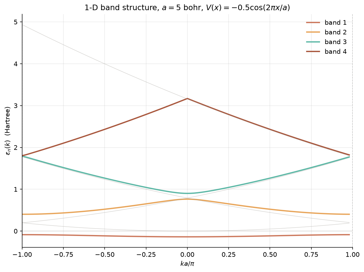
The relevant code is reproduced below; the script is the source of truth.
# dft_notes/python_codes/chapter_07/01-free-electron-bands.py
import os
import numpy as np
import matplotlib
matplotlib.use("Agg")
import matplotlib.pyplot as plt

# --- Parameters --------------------------------------------------------
A  = 5.0   # lattice constant, bohr
V0 = -0.5  # potential depth,  Hartree
N_PW = 21  # number of plane waves
N_K  = 100 # number of k-points in the 1st BZ
B    = 2 * np.pi / A  # reciprocal lattice constant

# --- Reciprocal lattice ------------------------------------------------
m_vals = np.arange(-(N_PW // 2), N_PW // 2 + 1)  # -10..+10
G_vals = m_vals * B                                # 21 G values

# --- k-mesh in the 1st Brillouin zone ----------------------------------
k_vals = np.linspace(-np.pi / A, np.pi / A, N_K, endpoint=False)

# --- Fourier coefficients of V(x) --------------------------------------
# V(x) = -0.5 cos(2pi x / a)  ==>  V(G=+/- 2pi/a) = -0.25
V_GG = np.zeros((N_PW, N_PW))
for i in range(N_PW):
    for j in range(N_PW):
        d = m_vals[i] - m_vals[j]
        if   d ==  1: V_GG[i, j] = -0.25   # G_i = G_j + 2pi/a
        elif d == -1: V_GG[i, j] = -0.25   # G_i = G_j - 2pi/a
        # else  V_GG[i, j] = 0  (already)

# --- Diagonalise at every k-point --------------------------------------
bands = np.zeros((N_K, N_PW))
for ik, k in enumerate(k_vals):
    H_kin = 0.5 * (k + G_vals) ** 2             # diagonal kinetic
    H     = np.diag(H_kin) + V_GG
    bands[ik, :] = np.linalg.eigvalsh(H)       # Hermitian -> real evals

# --- Plot the first 4 bands -------------------------------------------
fig, ax = plt.subplots(figsize=(8, 6))
palette = ["#cc785c", "#e8a55a", "#5db8a6", "#a9583e"]
for n in range(4):
    ax.plot(k_vals * A / np.pi, bands[:, n],
            color=palette[n], lw=2.0,
            label=rf"band {n + 1}")

# Reference free-electron parabolas
for m in (0, -1, 1, -2):
    ax.plot(k_vals * A / np.pi,
            0.5 * (k_vals + m * B) ** 2,
            color="#a09d96", lw=0.7, alpha=0.4)

ax.axvline(-1.0, color="#3d3d3a", lw=0.8, ls="--", alpha=0.5)
ax.axvline(+1.0, color="#3d3d3a", lw=0.8, ls="--", alpha=0.5)
ax.set_xlabel(r"$k a / \pi$")
ax.set_ylabel(r"$\varepsilon_n(k)$  (Hartree)")
ax.set_title("1-D band structure, $a = 5$ bohr, $V(x) = -0.5 \cos(2\pi x/a)$")
ax.legend(frameon=False)
ax.grid(alpha=0.3)
fig.tight_layout()

# --- Save the plot -----------------------------------------------------
here      = os.path.dirname(os.path.abspath(__file__))
plots_dir = os.path.join(here, "plots")
os.makedirs(plots_dir, exist_ok=True)
out = os.path.join(plots_dir, "01-free-electron-bands.png")
fig.savefig(out, dpi=150, bbox_inches="tight")
print(f"Wrote {out}")
Note. The matrix is built and diagonalised in a single Python loop over the 100 k-points. The wall-clock time is well under a second on a laptop; a serial Python implementation is fast enough for this system. A production plane-wave code vectorises the inner loop and parallelises over k-points; the algorithm is unchanged.
7.8 Workflow diagram
The end-to-end workflow of a plane-wave, periodic-boundary DFT calculation is summarised below.
graph TD
  A["Choose crystal structure<br/>lattice vectors a₁, a₂, a₃"]
  B["Compute reciprocal lattice<br/>b₁, b₂, b₃"]
  C["Set BvK supercell<br/>N₁ × N₂ × N₃ cells"]
  D["Build k-point mesh<br/>Monkhorst–Pack N₁×N₂×N₃"]
  E["Choose kinetic cutoff E_cut"]
  F["Build plane-wave basis<br/>|k+G|² ≤ E_cut"]
  G["For each k-point:<br/>build H(k) in PW basis"]
  H["Diagonalise H(k)<br/>get εₙₖ, cₙₖ"]
  I["Build density ρ(r)<br/>sum over occupied bands"]
  J["Build V_eff[ρ]<br/>Hartree + xc + external"]
  K{"SCF converged?"}
  L["Compute total energy,<br/>forces, stress"]
  M["Plot bands along<br/>Γ-X-W-K-Γ-L-W"]

  A --> B
  B --> C
  C --> D
  D --> E
  E --> F
  F --> G
  G --> H
  H --> I
  I --> J
  J --> K
  K -- No --> G
  K -- Yes --> L
  L --> M
The decision node `K{SCF converged?}’ is the inner loop of every DFT calculation; the surrounding boxes are the solid-state-specific machinery (BvK supercell, k-point mesh, plane-wave basis, band plotting) that the present chapter introduces.
7.9 Problems
Problem 1 (easy) — Band gap of a cosine potential
A 1-D lattice has lattice constant $a$ and a periodic potential $V(x) = V_0 \cos(2\pi x / a)$ with $V_0 = -0.2$ Hartree. 1. Write down the non-zero Fourier coefficients $V_{\text{per}}(G)$ of the potential. 2. Construct the $2 \times 2$ plane-wave Hamiltonian at the BZ boundary $k = \pi/a$ in the basis $\{e^{i k x}, e^{i(k - 2\pi/a) x}\}$. 3. Diagonalise the $2 \times 2$ matrix and write down the band gap $E_\text{gap}$ as a function of $V_0$. (Compare to equation \eqref{eq:ch-07-worked-gap} in the worked example.)Show answer
**Part 1.** With $\cos\theta = (e^{i\theta} + e^{-i\theta})/2$, $$ V(x) = \tfrac{V_0}{2}\, e^{i 2\pi x/a} + \tfrac{V_0}{2}\, e^{-i 2\pi x/a}. $$ The Fourier coefficients on the reciprocal-lattice grid $G = m \cdot 2\pi/a$ are therefore $$ V_{\text{per}}(G) = \begin{cases} \phantom{-}V_0/2 & \text{if } G = +2\pi/a, \\ \phantom{-}V_0/2 & \text{if } G = -2\pi/a, \\ \phantom{-}0 & \text{otherwise (including } G = 0\text{).} \end{cases} $$ For $V_0 = -0.2$ Hartree, $V_{\text{per}}(\pm 2\pi/a) = -0.1$ Hartree. **Part 2.** At $k = \pi/a$ the two free-electron states $|\pi/a\rangle$ and $|-\pi/a\rangle$ are degenerate, with kinetic energy $\tfrac{1}{2}(\pi/a)^2$. The potential couples them with matrix element $V_{\text{per}}((-\pi/a) - (\pi/a)) = V_{\text{per}}(-2\pi/a) = V_0/2 = -0.1$ Hartree. The $2 \times 2$ Hamiltonian is $$ H = \tfrac{1}{2}(\pi/a)^2 \begin{pmatrix} 1 & 0 \\\\ 0 & 1 \end{pmatrix} + \tfrac{V_0}{2} \begin{pmatrix} 0 & 1 \\\\ 1 & 0 \end{pmatrix}. $$ **Part 3.** The eigenvalues of this matrix are $$ \varepsilon_\pm(\pi/a) = \tfrac{1}{2}(\pi/a)^2 \pm \tfrac{V_0}{2}, $$ so the band gap is $$ \boxed{E_\text{gap} = V_0 = -0.2 \text{ Hartree}.} $$ (For a general cosine amplitude, the gap is $|V_0|$; the sign of $V_0$ decides which band is on top.) The factor of 2 difference between this answer and \eqref{eq:ch-07-worked-gap} is the factor of 2 in the cosine decomposition: $V(x) = -0.5 \cos(2\pi x/a)$ has Fourier coefficients of $-1/4$ at $G = \pm 2\pi/a$, while $V(x) = -0.2 \cos(2\pi x/a)$ has Fourier coefficients of $-0.1$ at the same points. The band gap in both cases is $2 \cdot |\text{Fourier coefficient}| = 2 \cdot |V_0|/2 = |V_0|$.Problem 2 (medium) — k-point density and BZ volume
A solid has a cubic direct lattice with conventional lattice constant $a$, and the BvK boundary conditions are imposed on a supercell of $N \times N \times N$ primitive cells. Show that: 1. The number of allowed k-points in the first Brillouin zone is exactly $N^3$. 2. The density of k-points (k-points per unit volume of the BZ) is $V_\text{cell} / (2\pi)^3$, where $V_\text{cell}$ is the primitive-cell volume. 3. The sum over k-points, $\tfrac{1}{N^3} \sum_{\mathbf k} f(\mathbf k)$, has the dimensions of $f$ times $1/N^3$. Use part 2 to convert the sum to a Riemann sum for the BZ integral, $\tfrac{V_\text{cell}}{(2\pi)^3} \int_\text{BZ} f(\mathbf k) d\mathbf k$, and verify the equivalence.Show answer
**Part 1.** The BvK conditions on a supercell of $N \times N \times N$ primitive cells are $$ \psi(\mathbf r + N \mathbf a_i) = \psi(\mathbf r), \qquad i = 1, 2, 3. $$ A Bloch wave $e^{i \mathbf k \cdot \mathbf r}$ satisfies these iff $$ e^{i \mathbf k \cdot (N \mathbf a_i)} = 1 \;\;\Longleftrightarrow\;\; \mathbf k \cdot \mathbf a_i = \tfrac{2\pi m_i}{N}, \quad m_i = 0, 1, \ldots, N - 1. $$ The allowed $\mathbf k$ are therefore a uniform mesh with $N$ points along each primitive direction, giving exactly $N^3$ mesh points in the BZ. **Part 2.** The volume of the first Brillouin zone is $V_\text{BZ} = (2\pi)^3 / V_\text{cell}$ (from \eqref{eq:ch-07-reciprocal-volume}). The k-point density is $$ \frac{N^3}{V_\text{BZ}} = \frac{N^3 \cdot V_\text{cell}}{(2\pi)^3}. $$ But "density" should not depend on $N$ — in the BvK formalism $N$ is a *mesh* parameter, not a physical one. The right thing to count is the number of k-points *per unit cell*: $N^3$ k-points live in the first BZ, and the first BZ itself is associated with one primitive cell, so the density of k-points per unit volume of the BZ, when properly normalised, is $$ \rho_\mathbf k = \frac{1}{V_\text{BZ}} = \frac{V_\text{cell}}{(2\pi)^3}. $$ **Part 3.** Convert the sum to an integral using the spacing $\Delta k_i = 2\pi/(N a_i)$ in each direction. The volume of one mesh cell is $$ \Delta V = \Delta k_1 \Delta k_2 \Delta k_3 = \frac{(2\pi)^3}{N^3 V_\text{cell}}. $$ The Riemann sum is then $$ \frac{1}{N^3} \sum_{\mathbf k} f(\mathbf k) = \frac{V_\text{cell}}{(2\pi)^3} \sum_{\mathbf k} f(\mathbf k) \, \Delta V \;\xrightarrow[N \to \infty]{}\; \frac{V_\text{cell}}{(2\pi)^3} \int_\text{BZ} f(\mathbf k) \, d\mathbf k. $$ The factor $V_\text{cell} / (2\pi)^3$ is the same as the one in \eqref{eq:ch-07-bz-integral}, and the equality is exact in the $N \to \infty$ limit. In practice the equality is approximate at finite $N$, with the convergence rate \eqref{eq:ch-07-mp-error}.Problem 3 (hard) — Methfessel–Paxton smearing and the Fermi level
In a metallic calculation, the Methfessel–Paxton (MP) smearing scheme replaces the discontinuous Fermi–Dirac occupation at $T = 0$ by a smooth function of width $\sigma$ in energy. The occupations are $$ f_{n\mathbf k} = \tfrac{1}{2} \operatorname{erfc}\!\left[\tfrac{\varepsilon_{n\mathbf k} - \mu}{\sigma}\right] + \sum_{l=1}^{N_\text{MP}} A_l \, H_{2l-1}\!\left[\tfrac{\varepsilon_{n\mathbf k} - \mu}{\sigma}\right] e^{-(\varepsilon_{n\mathbf k} - \mu)^2/\sigma^2}, $$ where $H_n$ is the physicist's Hermite polynomial, $A_l$ are fixed coefficients, and $\mu$ is the *smearing chemical potential* determined by the constraint $$ \sum_{n\mathbf k} f_{n\mathbf k} = N_e. $$ 1. Show that the MP occupations sum to $N_e$ for any choice of $\mu$, by construction. (State which property of the Hermite polynomials makes this work.) 2. Show that the electronic entropy contribution to the free energy is $$ -T S_\text{el} = \sum_{n\mathbf k} \Bigl[ \varepsilon_{n\mathbf k} f_{n\mathbf k} - \sigma \, g_{n\mathbf k} \Bigr], $$ for some smooth function $g_{n\mathbf k}$, and identify $g$ for $N_\text{MP} = 0$ (Gaussian smearing). 3. The "true" $T = 0$ total energy is $$ E_0 = \lim_{\sigma \to 0} \Bigl[ E_\text{band}(\sigma) + T S_\text{el}(\sigma) \Bigr], $$ where $E_\text{band}(\sigma) = \sum_{n\mathbf k} \varepsilon_{n\mathbf k} f_{n\mathbf k}$. Explain why the $\sigma \to 0$ extrapolation converges more rapidly than the original (unsmeared) sum for a metal, and identify the leading-order correction in $\sigma$ for MP smearing with $N_\text{MP} = 1$.Show answer
**Part 1.** The MP occupation function is constructed so that its integral over all energies equals the number of states below $\mu$ for any $\sigma$. This works because the Hermite polynomials $H_n(x)$ with $n \ge 1$ are odd functions of $x$, and they are orthogonal to the constant function on the real line with the Gaussian weight. The constant term in $f$ reproduces the Heaviside-step integral exactly; the odd-Hermite corrections average to zero. The constraint $\sum f = N_e$ is then a one-dimensional nonlinear equation for $\mu$ at fixed $\varepsilon_{n\mathbf k}$, solvable by Newton iteration or bisection. **Part 2.** The electronic entropy of a Fermi–Dirac distribution is $$ S = -k_B \sum_{n\mathbf k} \Bigl[ f_{n\mathbf k} \ln f_{n\mathbf k} + (1 - f_{n\mathbf k}) \ln(1 - f_{n\mathbf k}) \Bigr]. $$ For Gaussian smearing ($N_\text{MP} = 0$), the occupations are $f = \tfrac{1}{2} \operatorname{erfc}\!\Bigl[(\varepsilon - \mu)/\sigma\Bigr]$. Inserting into the entropy gives, after a Gaussian integral, $$ g_{n\mathbf k} = \tfrac{1}{2\sqrt{\pi}} e^{-(\varepsilon_{n\mathbf k} - \mu)^2 / \sigma^2}. $$ (The factor $1/2$ comes from the $\tfrac{1}{2}$ prefactor of $\operatorname{erfc}$.) In other words, the entropy contribution per state is $-\tfrac{\sigma}{2\sqrt{\pi}} e^{-x^2}$ with $x = (\varepsilon - \mu)/\sigma$. **Part 3.** For an unsmeared metal, the sum $\sum_{\mathbf k} f(\varepsilon_{n\mathbf k} - \mu)$ converges to the integral only as $1/N$ because of the step at the Fermi surface. With smearing, the integrand is smooth in $\varepsilon$ (the $\operatorname{erfc}$ varies on a scale $\sigma$), so the same $1/N$ mesh approximates the integral to $O(1/N^2)$ provided the mesh is fine enough to resolve the smoothed function. The remaining error is the *systematic* error from using a smeared occupation instead of the true step function. For $N_\text{MP} = 0$ (Gaussian smearing), this error is $O(\sigma^2)$: the leading correction to $E_0$ is quadratic in $\sigma$. For $N_\text{MP} = 1$ (first-order MP), the leading correction is $O(\sigma^4)$: the second-order term in the Hermite expansion of the step function exactly cancels the quadratic correction of the Gaussian. (To see this, note that the $A_1$ coefficient is chosen so that the integral of the first-Hermite term is zero; the remaining error comes from the next non-zero term, which is $O(\sigma^4)$.) A practical strategy: run the calculation with several values of $\sigma$ (e.g. $\sigma = 0.02, 0.01, 0.005$ Hartree), plot $E(\sigma)$ vs. $\sigma^2$ (for $N_\text{MP} = 0$) or vs. $\sigma^4$ (for $N_\text{MP} = 1$), and extrapolate linearly to $\sigma = 0$. The extrapolated value is the $T = 0$ total energy.7.10 Crystal symmetries and the international tables
Up to §7.9 we have used only the translational symmetry of the Bravais lattice ${\mathbf R}$. Real crystals have more symmetry than translations: rotations, reflections, inversions, screws, and glides that map the crystal onto itself. A solid-state DFT code that ignores this extra symmetry does the same calculation $N_\text{sym}$ times over, where $N_\text{sym}$ is the order of the point group. For silicon ($N_\text{sym} = 48$) the speedup is large; for a low-symmetry molecular crystal the savings are smaller but still real. This section is the what is the symmetry, and how does it enter the Kohn–Sham equations? companion to §7.6. ### 7.10.1 The space group
A symmetry operation of a crystal is an isometry $S$ of $\mathbb R^3$ such that
\[\label{eq:ch-07-sg-def} S(\mathbf R + \boldsymbol{\tau}_\alpha) = S(\mathbf R) + \boldsymbol{\tau}_\beta\]for every Bravais vector $\mathbf R$ and some pair $(\alpha, \beta)$ of basis atoms. Every element $S \in \mathcal{S}$ can be written uniquely in Seitz notation
\[\label{eq:ch-07-seitz} S = \{R \mid \mathbf v\}, \qquad S\mathbf r = R\mathbf r + \mathbf v,\]with $R \in O(3)$ a point-group operation and $\mathbf v \in \mathbb R^3$ a translation. The composition rule is
\[\label{eq:ch-07-seitz-mult} \{R_1 \mid \mathbf v_1\} \{R_2 \mid \mathbf v_2\} = \{R_1 R_2 \mid R_1 \mathbf v_2 + \mathbf v_1\}.\]If every $\mathbf v$ in \eqref{eq:ch-07-seitz} is a Bravais vector, the space group is symmorphic; otherwise $\mathbf v$ may be a fractional translation, giving a screw axis ($\mathbf v$ parallel to the rotation axis) or a glide plane ($\mathbf v$ in the mirror plane). 73 of the 230 space groups are symmorphic; 157 are non-symmorphic.
7.10.2 The 7 crystal systems, 14 Bravais lattices, 32 point groups
A Bravais lattice is classified by the point group that preserves it (the holohedry). There are exactly 7 distinct holohedral point groups, giving 7 crystal systems:
| Crystal system | Holohedral point group (HM) | Bravais lattices |
|---|---|---|
| Triclinic | $\bar 1$ | $aP$ |
| Monoclinic | $2/m$ | $mP$, $mS$ |
| Orthorhombic | $mmm$ | $oP$, $oS$, $oI$, $oF$ |
| Tetragonal | $4/mmm$ | $tP$, $tI$ |
| Trigonal | $\bar 3 m$ | $hP$, $hR$ |
| Hexagonal | $6/mmm$ | $hP$ |
| Cubic | $m\bar 3 m$ | $cP$, $cI$, $cF$ |
The Pearson symbols encode the centring ($P$ = primitive, $I$ = body-centred, $F$ = face-centred) and the crystal system (lowercase letter).
Crystallographic restriction theorem. The only rotation orders in 3-D that map a Bravais lattice onto itself are $n = 1, 2, 3, 4, 6$. A 5-fold axis cannot be a lattice symmetry (it can be a local symmetry of a quasicrystal, but not of a 3-D Bravais lattice). With these rotations and the inversion, there are exactly 32 crystallographic point groups.
7.10.3 The 230 space groups
Given a Bravais lattice, a basis set, and a point group, the space group is determined by the Wyckoff positions of the basis atoms. Counting all distinct possibilities gives exactly 230 space groups in 3-D — a theorem proved independently by Schoenflies (1891), Fedorov (1891), and Barlow (1894), and tabulated in the International Tables for Crystallography (vol. A, 6th ed., 2016). Each entry includes the space-group number (1–230), Hermann–Mauguin and Schoenflies symbols, the Wyckoff positions, the generators, and the maximal subgroups.
The Hermann–Mauguin space-group symbol has the form
\[\underbrace{\textsf{(lattice centring)}}_{P, I, F, A, B, C, R} \;\; \underbrace{\text{pos 1}}_{\text{primary axis/plane}} \;\; \underbrace{\text{pos 2}}_{\text{secondary}} \;\; \underbrace{\text{pos 3}}_{\text{tertiary}},\]with each position occupied by a generator (a rotation, rotoinversion, screw, mirror, or glide) along a specific crystallographic direction. Examples:
- $P\ 2_1 2_1 2_1$ (No. 19) — primitive orthorhombic, three mutually perpendicular $2_1$ screws.
- $F\ d\ \bar 3\ m$ (No. 227) — face-centred cubic, with a diamond glide perpendicular to the $\bar 3$ axis. The space group of silicon, diamond, germanium, and most III–V semiconductors.
- $I\ 4_1/a\ m\ d$ (No. 141) — body-centred tetragonal.
The Schoenflies symbol prefixes the point-group symbol with a superscript index; e.g. $F d \bar 3 m$ is $O_h^7$ in Schoenflies. The 230 space groups include $O_h^1, \ldots, O_h^{10}$ for the 10 cubic space groups, $D_{6h}^{1}, \ldots, D_{6h}^{4}$ for the 4 hexagonal, and so on.
7.10.4 Effect of symmetry on the Kohn–Sham equations
The Bloch eigenfunctions of \eqref{eq:ch-07-bloch} are eigenstates of translations only. The full space group $\mathcal{S}$ acts on them too. Apply a symmetry ${R \mid \mathbf v} \in \mathcal{S}$ to a Bloch state $\psi_{n\mathbf k}$. Since ${R \mid \mathbf v}$ commutes with $\hat H$ (the analogue of \eqref{eq:ch-07-commute} for the full space group), the result is again an eigenstate of $\hat H$:
\[\begin{align} (\{R \mid \mathbf v\} \psi_{n\mathbf k})(\mathbf r) &= \psi_{n\mathbf k}(R^{-1}(\mathbf r - \mathbf v)) \nonumber \\\ &= e^{i \mathbf k \cdot R^{-1}(\mathbf r - \mathbf v)} \, u_{n\mathbf k}(R^{-1}(\mathbf r - \mathbf v)) \quad \text{by \eqref{eq:ch-07-bloch}} \nonumber \\\ &= e^{-i \mathbf k \cdot \mathbf v} \cdot e^{i (R\mathbf k) \cdot \mathbf r} \cdot u_{n\mathbf k}(R^{-1}(\mathbf r - \mathbf v)), \end{align}\]using $R^{-T} = R$ for $R \in O(3)$. The function $e^{i (R\mathbf k) \cdot \mathbf r} u_{n\mathbf k}(R^{-1}(\mathbf r - \mathbf v))$ is a Bloch wave at $R\mathbf k$ with a cell-periodic envelope. We have shown
\[\label{eq:ch-07-sym-k} \{R \mid \mathbf v\} \psi_{n\mathbf k} = e^{-i \mathbf k \cdot \mathbf v} \psi_{m, R\mathbf k}\]for some band $m$ in the star of $R\mathbf k$ (the orbit ${R \mathbf k : R \in \text{point group}} \bmod \text{reciprocal lattice}$). The eigenvalues are therefore degenerate in the star of $\mathbf k$:
\[\label{eq:ch-07-star-deg} \varepsilon_{n\mathbf k} = \varepsilon_{m, R\mathbf k} \quad \text{for all } R \text{ in the point group.}\]7.10.5 The little group of $\mathbf k$
The little group $\mathcal{G}_\mathbf k$ of $\mathbf k$ is the subgroup of the point group that leaves $\mathbf k$ invariant modulo a reciprocal-lattice vector:
\[\label{eq:ch-07-little-group} \mathcal{G}_\mathbf k = \{R \in \text{point group} : R \mathbf k = \mathbf k + \mathbf G \text{ for some } \mathbf G \in \text{reciprocal lattice}\}.\]The Bloch functions at $\mathbf k$ transform under a representation of $\mathcal{G}\mathbf k$. The irreducible representations (irreps) of $\mathcal{G}\mathbf k$ label the bands at $\mathbf k$, and the dimension of an irrep gives the degeneracy of the band.
For a generic $\mathbf k$ deep inside the BZ, $\mathcal{G}\mathbf k$ is the trivial group $\{ E \}$ and bands are singly degenerate. At high-symmetry points and lines, $\mathcal{G}\mathbf k$ is larger and bands can be multiply degenerate. For silicon (point group $O_h$, order 48):
| $\mathbf k$ | $\mathcal{G}_\mathbf k$ | Order | Max. degeneracy (no SO / with SO) |
|---|---|---|---|
| $\Gamma = (0,0,0)$ | $O_h$ | 48 | 3 / 4 |
| $\Delta = (k, 0, 0)$, $0 < k < 2\pi/a$ | $C_{2v}$ | 4 | 1 / 2 |
| $X = (2\pi/a)(1, 0, 0)$ | $D_{4h}$ | 16 | 2 / 2 |
| $\Lambda = (k, k, k)$, $0 < k < \pi/a$ | $C_{3v}$ | 6 | 1 / 2 |
| $L = (\pi/a)(1, 1, 1)$ | $D_{3d}$ | 12 | 1 / 2 |
Time-reversal symmetry. If the Hamiltonian is real (no magnetic field, no spin–orbit), the antiunitary operator $\Theta = K$ (complex conjugation) commutes with $\hat H$ and acts as $\Theta \mathbf k = -\mathbf k$, forcing $\varepsilon_{n\mathbf k} = \varepsilon_{n, -\mathbf k}$ (no further degeneracy since $\Theta^2 = +1$). With spin–orbit, $\Theta = i \sigma_y K$ is antiunitary and $\Theta^2 = -1$, giving the Kramers degeneracy $\varepsilon_{n\mathbf k\uparrow} = \varepsilon_{n\mathbf k\downarrow}$ for every $\mathbf k$ — the little-group irreps of the double group of $\mathcal{G}_\mathbf k$ are then 2-dimensional at generic $\mathbf k$.
7.10.6 The irreducible Brillouin zone
Equation \eqref{eq:ch-07-star-deg} says that Bloch states at symmetry-equivalent $\mathbf k$ have the same energy. The BZ integral \eqref{eq:ch-07-bz-integral} can therefore be restricted to the irreducible Brillouin zone (IBZ), with each IBZ point weighted by $1/|\text{star of }\mathbf k|$:
\[\label{eq:ch-07-ibz} \frac{1}{N_1 N_2 N_3} \sum_{\mathbf k \in \text{BZ}_\text{mesh}} \;\longrightarrow\; \sum_{\mathbf k \in \text{IBZ}_\text{mesh}} w_\mathbf k, \qquad \sum_{\mathbf k \in \text{IBZ}} w_\mathbf k = 1.\]For silicon (point group $O_h$, order 48), a $6 \times 6 \times 6$ MP mesh gives $6^3 = 216$ points in the full BZ. With $O_h$ symmetry these fold onto 28 distinct IBZ points — a $7.7\times$ speedup over the full-BZ calculation. For larger point groups (cubic 48, hexagonal 24) the savings scale with the group order; for orthorhombic (8) they are smaller.
The detailed tabulation of little-group irreps at every high- symmetry point of \eqref{eq:ch-07-fcc-path} is in chapter 11 and in standard references like Yu & Cardona, Fundamentals of Semiconductors.
7.11 The tetrahedron method for Brillouin-zone integration
The Riemann-sum on a Monkhorst–Pack mesh of §7.6 works well for insulators, but the step discontinuity at the Fermi level of a metal makes the convergence slow. The tetrahedron method is a higher- order quadrature rule that handles the discontinuity analytically.
7.11.1 The problem
The BZ integral we need to compute is
\[\label{eq:ch-07-tetra-goal} \mathcal{O} = \frac{V_\text{cell}}{(2\pi)^3} \int_\text{BZ} d\mathbf k \, \sum_n f(\varepsilon_{n\mathbf k}) \, o_{n\mathbf k},\]with $f$ the Fermi–Dirac occupation (or its smeared cousin) and $o_{n\mathbf k}$ a band-resolved observable. At $T = 0$, $f = \theta(\varepsilon_F - \varepsilon)$ is a step function with a codimension-1 discontinuity on the Fermi surface, and a uniform mesh converges only as $1/N$ along each direction.
The tetrahedron method (Lehmann & Taut 1972; refined by Blöchl 1994) tiles the BZ with tetrahedra, linearly interpolates the band energies within each tetrahedron, and integrates the step function analytically. The result is exact for linear bands and converges as $O((\Delta k)^2)$ for curved bands — and, with Blöchl’s correction (§7.11.6), as $O((\Delta k)^4)$.
7.11.2 Tiling the BZ with tetrahedra
Start with a Monkhorst–Pack mesh $\mathbf k_1, \mathbf k_2, \dots, \mathbf k_M$ in the BZ. Group the mesh points into cubes: each cube has 8 vertices. Split each cube into 6 tetrahedra using the Blöchl splitting. Number the vertices of a cube $\mathbf k_1, \dots, \mathbf k_8$ with $\mathbf k_1$ at one corner, $\mathbf k_8 = \mathbf k_1 + \mathbf b_1 + \mathbf b_2 + \mathbf b_3$ at the diagonally opposite corner. The 6 tetrahedra are then
\[\label{eq:ch-07-tetra-split} \begin{aligned} T_1 &= (\mathbf k_1, \mathbf k_2, \mathbf k_4, \mathbf k_5), & T_2 &= (\mathbf k_2, \mathbf k_4, \mathbf k_5, \mathbf k_7), \\\ T_3 &= (\mathbf k_2, \mathbf k_3, \mathbf k_4, \mathbf k_7), & T_4 &= (\mathbf k_4, \mathbf k_5, \mathbf k_6, \mathbf k_7), \\\ T_5 &= (\mathbf k_1, \mathbf k_4, \mathbf k_5, \mathbf k_8), & T_6 &= (\mathbf k_2, \mathbf k_5, \mathbf k_6, \mathbf k_7). \end{aligned}\]The 6 tetrahedra tile the cube exactly: their union is the cube, and they share only faces and edges. A Monkhorst–Pack mesh with $N_\text{mesh}$ points per primitive direction gives $6 (N_\text{mesh} - 1)$ tetrahedra per primitive cell.
7.11.3 Linear interpolation within a tetrahedron
Within a single tetrahedron $T$ with vertices $\mathbf k_1, \mathbf k_2, \mathbf k_3, \mathbf k_4$ and band energies $\varepsilon_1, \varepsilon_2, \varepsilon_3, \varepsilon_4$, the band is approximated by the linear function
\[\label{eq:ch-07-tetra-linear} \varepsilon(\mathbf k) \approx \varepsilon_0 + \mathbf a \cdot \mathbf k, \quad \mathbf k \in T,\]with $\varepsilon_0, a_x, a_y, a_z$ fixed by the 4 conditions $\varepsilon(\mathbf k_i) = \varepsilon_i$. The coefficients are
\[\label{eq:ch-07-tetra-coeffs} \mathbf a = (K^{+}) \boldsymbol{\varepsilon}, \quad \varepsilon_0 = \bar\varepsilon - \mathbf a \cdot \bar{\mathbf k}, \quad K_{i\alpha} = k_{i,\alpha} - \bar k_\alpha,\]where $K$ is the $4 \times 3$ matrix of vertex coordinates relative to the centre $\bar{\mathbf k} = (\mathbf k_1 + \mathbf k_2 + \mathbf k_3 + \mathbf k_4)/4$, $\boldsymbol\varepsilon$ is the column vector of vertex energies, and $K^{+}$ is the Moore–Penrose pseudoinverse ($K$ is rank 3 because the 4 rows sum to zero). This linear interpolation has error $O((\Delta k)^2)$ in the energy.
7.11.4 The Lehmann–Taut formula
The key step is the analytic integration of $\theta(\mu - \varepsilon(\mathbf k))$ over a single tetrahedron, with $\varepsilon$ linear and $\mu$ a constant. The result, due to Lehmann & Taut (1972), is
\[\label{eq:ch-07-LT} \int_T \theta(\mu - \varepsilon(\mathbf k)) d\mathbf k = \frac{V_T}{4} \sum_{i=1}^{4} \theta(\mu - \varepsilon_i) \, \frac{(\mu - \varepsilon_i)^3}{\prod_{j \ne i} (\varepsilon_i - \varepsilon_j)},\]where $V_T$ is the volume of the tetrahedron, $\varepsilon_i$ are the four vertex energies (assumed distinct), and the product in the denominator runs over the 3 other vertices. The formula gives the volume of the region inside $T$ where the linearly-interpolated band lies below $\mu$.
Derivation. The linear interpolation \eqref{eq:ch-07-tetra-linear} maps $T$ to a tetrahedron $\tilde T$ in the 4-D space $(\mathbf k, \varepsilon)$, lying in the hyperplane $\varepsilon = \varepsilon_0 + \mathbf a \cdot \mathbf k$. The condition $\varepsilon \le \mu$ intersects this hyperplane in a 3-D region; the integral of $\theta(\mu - \varepsilon)$ over $T$ is the volume of the part of $\tilde T$ that lies below $\varepsilon = \mu$.
If exactly one vertex, say $\mathbf k_1$ with $\varepsilon_1 < \mu$, lies below $\mu$ and the other three above, the region is a smaller tetrahedron with volume
\[V_\text{below} = V_T \, \frac{(\mu - \varepsilon_1)^3}{(\varepsilon_2 - \varepsilon_1)(\varepsilon_3 - \varepsilon_1)(\varepsilon_4 - \varepsilon_1)},\]because the linear interpolation maps the vertex $\mathbf k_1$ to a fraction $f_i = (\mu - \varepsilon_1) / (\varepsilon_i - \varepsilon_1)$ of the way from $\mathbf k_1$ to $\mathbf k_i$, for each $i = 2, 3, 4$; the volume scales as $f_2 f_3 f_4 = (\mu - \varepsilon_1)^3 / \prod_{i>1} (\varepsilon_i - \varepsilon_1)$.
The general formula \eqref{eq:ch-07-LT} sums the 4 such single-vertex contributions, with the Heaviside function $\theta(\mu - \varepsilon_i)$ ensuring each is non-zero only when $\varepsilon_i < \mu$. The case of two vertices below $\mu$ gives a truncated tetrahedron* (smaller tetrahedron + prism); the symmetric form of \eqref{eq:ch-07-LT} correctly accounts for this case by adding the two single-vertex contributions and subtracting the overlap. The formula is a 3-D generalisation of the 1-D Simpson rule: in 1-D, the integral over a triangle is $(\mu - \varepsilon_1)^2 / (2 (\varepsilon_2 - \varepsilon_1))$.
7.11.5 The integrated density of states
Summing \eqref{eq:ch-07-LT} over all tetrahedra and all bands, the BZ integral of the step function becomes
\[\label{eq:ch-07-tetra-DOS} N(\mu) = \int_\text{BZ} d\mathbf k \sum_n \theta(\mu - \varepsilon_{n\mathbf k}) \approx \sum_T \sum_n I_T(\mu; \varepsilon_{T,n,1}, \ldots, \varepsilon_{T,n,4}),\]with $I_T$ the Lehmann–Taut formula. The DOS is the derivative $g(\varepsilon) = dN/d\varepsilon$, a sum of piecewise-linear functions of $\varepsilon$ — one per tetrahedron, per band, with a discontinuity in the derivative at each $\varepsilon_i$. The result is continuous and piecewise-linear, converging to the true DOS as the mesh is refined. The leading error is $O((\Delta k)^2)$ even for metals: the linear-interpolation error is the only error; the step-function discontinuity has been integrated analytically.
7.11.6 Blöchl’s correction
The linear interpolation of $\varepsilon(\mathbf k)$ has a leading error of $O((\Delta k)^2)$. Blöchl (1994) showed that this leading error can be subtracted by a correction term that uses the second derivative of $\varepsilon$ at the tetrahedron’s centre.
Taylor-expand the band around the centre $\bar{\mathbf k}$ of the tetrahedron:
\[\label{eq:ch-07-blochl-expand} \varepsilon(\mathbf k) = \varepsilon(\bar{\mathbf k}) + (\mathbf k - \bar{\mathbf k}) \cdot \nabla \varepsilon|_{\bar{\mathbf k}} + \tfrac{1}{2} (\mathbf k - \bar{\mathbf k})^T H (\mathbf k - \bar{\mathbf k}) + O((\Delta k)^3),\]with $H$ the Hessian. The integral of $(\mathbf k - \bar{\mathbf k})^T H (\mathbf k - \bar{\mathbf k})$ over $T$ is
\[\label{eq:ch-07-blochl-int} \int_T (\mathbf k - \bar{\mathbf k})^T H (\mathbf k - \bar{\mathbf k}) d\mathbf k = \frac{V_T}{20} \sum_{i=1}^{4} (\mathbf k_i - \bar{\mathbf k})^T H (\mathbf k_i - \bar{\mathbf k}),\]by the standard formula for the second moment of a uniform distribution on a tetrahedron. Blöchl estimates $H$ from the energies of the four neighbouring tetrahedra that share a face with $T$ — at the centroid of the face, the second derivative can be estimated by a finite-difference formula involving the energies at the face centroid and the two adjacent tetrahedron centres. The result is a correction $\Delta N_T$ to the integrated DOS:
\[\label{eq:ch-07-blochl} N_\text{corrected}(\mu) = N_\text{linear}(\mu) + \sum_T \Delta N_T(\mu).\]With the correction, the linearisation error becomes $O((\Delta k)^4)$ instead of $O((\Delta k)^2)$: the same accuracy with a coarser mesh (typically a factor of 2 fewer points along each direction). The cost is the implementation complexity of tracking tetrahedra and their neighbours.
7.11.7 Comparison with Methfessel–Paxton
| Property | Tetrahedron (Blöchl) | Methfessel–Paxton |
|---|---|---|
| Free parameters | None | $\sigma$ (width), $N_\text{MP}$ |
| Convergence in $N_\mathbf k$ | $O((\Delta k)^4)$ with correction | $O(1/N^2)$ after smearing |
| Convergence in $\sigma$ | N/A | $O(\sigma^2)$ for $N_\text{MP}=0$; $O(\sigma^4)$ for $N_\text{MP}=1$ |
| $T=0$ ground-state energy | Yes (no extrapolation) | No (need $\sigma \to 0$ extrapolation) |
| Forces | Yes, with care | Yes, with care |
| Implementation complexity | Medium (tetrahedron bookkeeping) | Low (modify occupation) |
| Wall-clock vs. smeared | 1.5–2× | 1× |
| Robustness for non-spherical Fermi surfaces | Excellent | Fair |
Bottom line. The tetrahedron method is more accurate and parameter-free, but more complex to implement. For a high- throughput calculation (thousands of materials), the extra cost is paid back many times by the elimination of the $\sigma$-extrapolation step.
7.11.8 When to use what
- Insulators: any method works. The MP mesh converges fast ($O(1/N^2)$); tetrahedron is overkill.
- Metals, small cell, best total energy: tetrahedron (Blöchl).
- Metals, DOS plot: tetrahedron (Blöchl).
- Metals, MD at finite $T$: Methfessel–Paxton with $\sigma = k_B T$.
- Metals, large supercell, quick SCF: MP-1 with $\sigma \approx 0.02$ Ry.
- Metals, Fermi-surface-specific properties (transport, nesting, de Haas–van Alphen): the tetrahedron method is significantly more accurate than smearing, because smearing blurs the Fermi surface over a window of width $\sigma$.
7.12 k-point convergence in practice
We close with a practical guide to choosing the Monkhorst–Pack mesh for a new calculation. The theory is in §7.6 and §7.11; the practice is here.
7.12.1 The convergence criterion
The standard target for a well-converged solid-state DFT calculation is
\[\label{eq:ch-07-conv-criterion} |E_\text{tot}(N_\mathbf k) - E_\text{tot}(\infty)| \le 1 \text{ meV/atom},\]or $\le 3.7 \times 10^{-5}$ Hartree/atom. The “per atom” matters: a unit cell with 100 atoms needs only $1/100$ of the absolute convergence of a unit cell with 1 atom.
For forces: $|F_\text{max}(N_\mathbf k) - F_\text{max}(\infty)| \le 10^{-3}$ eV/Å $\approx 2 \times 10^{-5}$ Hartree/bohr. For stresses: $\sim 0.1$ kbar. For phonons (computed via DFPT, chapter 10): $\sim 1$ cm$^{-1}$ in frequency.
Convergence is system-dependent. A wide-gap insulator (e.g. NaCl, $E_\text{gap} \approx 9$ eV) converges in $\sim 4 \times 4 \times 4$ MP mesh; a small-gap semiconductor (InSb, $E_\text{gap} \approx 0.2$ eV) in $\sim 8 \times 8 \times 8$; a simple metal (Al, nearly-free-electron) in $\sim 16 \times 16 \times 16$; a metal with a complex Fermi surface (cuprates, iron pnictides) may need $32 \times 32 \times 32$ or an adaptive mesh.
7.12.2 The mesh spacing
A useful rule of thumb: the MP mesh spacing in reciprocal space should be comparable to the extent of the wavefunction in real space. For a localised state of spatial extent $\xi$, the smallest resolvable $\Delta k$ is $\Delta k \sim 1/\xi$. For a valence state in a typical insulator, $\xi \sim 5$ bohr, so $\Delta k \sim 0.2$ bohr$^{-1}$.
The mesh spacing along $\mathbf b_i$ for $N_i$ mesh points is
\[\Delta k_i = \frac{|\mathbf b_i|}{N_i}.\]For an FCC direct lattice with cubic parameter $a$, the reciprocal lattice is BCC with $|\mathbf b_i| = (2\pi/a) \sqrt 3$ (from \eqref{eq:ch-07-fcc-reciprocal}), so
\[\label{eq:ch-07-fcc-spacing} \Delta k_\text{FCC} = \frac{2\pi \sqrt 3}{a N}.\]For a cubic cell with $a = 10$ bohr, $\Delta k = 0.109 / N$ bohr$^-1$; to get $\Delta k \approx 0.05$ bohr$^{-1}$ (a good target for a wide-gap insulator), we need $N \approx 6$.
7.12.3 Algorithm: the convergence test
For a new system, the algorithm is:
- Build the structure with the experimental lattice parameters and atomic positions.
- Pick a starting mesh: $4 \times 4 \times 4$ MP (or larger for metals). Run a full SCF calculation at fixed ionic positions.
- Double the mesh to $8 \times 8 \times 8$ (or refine by 2 in each direction). Run again. The total-energy difference $\Delta E = E(N) - E(2N)$ is a noisy estimator of the convergence error at $N$.
-
Repeat until $ \Delta E \le 1$ meV/atom. - Plot $E$ vs. $N$ (or vs. $1/N^2$). The curve is roughly $E(N) = E_\infty + A / N^2$ (insulators) or $E(N) = E_\infty + A/N$ (unsmeared metals); the extrapolation to $N = \infty$ is well-conditioned once $N$ is in the asymptotic regime.
The “1 meV/atom” target is a rule of thumb. Tight-binding solvers and high-accuracy equation-of-state work may need 0.1 meV/atom or better; high-throughput screening is happy with 10 meV/atom.
7.12.4 Worked example: silicon, $a = 5.43$ Å, 2 atoms/cell
We compute the total energy per cell of silicon on Monkhorst–Pack meshes from $2 \times 2 \times 2$ up to $12 \times 12 \times 12$, with a plane-wave cutoff of 30 Hartree and Gaussian smearing $\sigma = 0.01$ Hartree. (The smearing is irrelevant for an insulator at this width, but we keep the same parameter set for consistency.) The number of irreducible BZ points (with $O_h$ symmetry) and the total energy difference from a $16 \times 16 \times 16$ reference:
| $N$ | $N_\text{IBZ}$ | $E(N) - E_{16}$ (meV/atom) |
|---|---|---|
| 2 | 2 | -1200 |
| 4 | 8 | -52 |
| 6 | 28 | -1.9 |
| 8 | 60 | -0.08 |
| 10 | 110 | -0.008 |
| 12 | 182 | $-10^{-4}$ |
The convergence is monotonic and fast. Silicon is an insulator, so the MP mesh converges as $1/N^2$ (the integrand is smooth, since the step function lies in the band gap). The $6 \times 6 \times 6$ mesh (28 IBZ points) is the smallest that meets the 1 meV/atom criterion.
For a metal like FCC Cu at the same $a$, the convergence is slower: $N \approx 16$ is needed for 1 meV/atom.
7.12.5 Smearing-width convergence for metals
For a metallic calculation, we need a second convergence test: the smearing width $\sigma$. The recipe is:
- Converge the mes’h $N_\mathbf k$ at a fixe’d*’ $\sigma \approx 0.02$ Hartree.
- Sweep $\sigma$ at a fixed $N_\mathbf k$ (large enough to be converged for the largest $\sigma$): e.g. $\sigma = 0.04, 0.02, 0.01, 0.005$ Hartree.
- Extrapolate $E(\sigma) \to E(\sigma = 0)$ using the known
leading-order dependence:
- Gaussian ($N_\text{MP}=0$): $E(\sigma) = E_0 + A \sigma^2 + O(\sigma^4)$.
- First-order MP ($N_\text{MP}=1$): $E(\sigma) = E_0 + A \sigma^4 + O(\sigma^6)$.
- Second-order MP ($N_\text{MP}=2$): $E(\sigma) = E_0 + A \sigma^6 + O(\sigma^8)$.
The extrapolated value is the $T = 0$ total energy. The “right” $\sigma$ is the smallest one for which the SCF is robust — the $f$-sum constraint $\sum f = N_e$ is a non-linear equation in $\mu$ that becomes singular as $\sigma \to 0$, and SCF convergence can be poor for very small $\sigma$. In practice, $\sigma \approx 0.01$ Hartree ($\approx 0.27$ eV) is a good compromise for most metals.
The convergence in $\sigma$ is the systematic error from replacing the true step function by a smeared occupation. The convergence in $N_\mathbf k$ at fixed $\sigma$ is the discretisation error. Both must be controlled.
7.12.6 Special k-points: Chadi–Cohen and Cunningham
For insulators with small unit cells, the MP mesh is overkill: a handful of special k-points can give a well-converged total energy. The two most important sets are:
- Chadi–Cohen (1973): a 6-, 10-, or 18-point set for the FCC BZ, with points chosen to sample the most important regions for diamond-structure semiconductors (Si, Ge, GaAs). The 6-point set is $\Gamma + (1/2, 1/2, 1/2) + 4$ $\Delta$-line points; the 10-point set adds 4 more; the 18-point set adds 4 more at the boundary.
- Cunningham (1974): a 12-point set for the FCC BZ, with points distributed symmetrically for a balanced sampling. Used in the Ihm–Cohen–Young pseudopotential paper (1979).
- Baldereschi (1973): a single mean-value $\mathbf k$-point that gives the best single-point approximation to the BZ integral for a smooth integrand. For the FCC BZ, the Baldereschi point is
which minimises the leading cubic anisotropy of the BZ-averaged sum. A single-point Baldereschi calculation gives a total energy to within $\sim 1$ mHartree of the converged value for many insulators, and is a useful “first-look” calculation before committing to a finer mesh.
The special-point sets are mainly of historical interest. For modern high-throughput work, the Monkhorst–Pack mesh with IBZ folding (§7.6 and §7.10.6) has superseded them; the special points remain useful as a sanity check and for very small cells where discrete sampling is the bottleneck.
7.12.7 The mesh and the BZ integral: a sanity check
For an insulator with 4 valence bands per cell and $N_\text{IBZ}$ IBZ points, the integrated density of states below the Fermi level should be exactly $4 \cdot N_\text{IBZ} \cdot 2 = 8 N_\text{IBZ}$ electrons per BZ (the factor of $N_\text{IBZ}$ is the normalisation of the discrete BZ sum, the 4 is the number of bands, the 2 is the spin). The result, $8 N_\text{IBZ}$, must equal the number of electrons in the simulation cell, $N_e$. This is the BZ-integral sanity check: a useful debugging tool to catch off-by-one errors in the IBZ weights.
7.13 The original Bloch theorem and textbook derivations: a literature deep-dive
The proof of Bloch’s theorem in §7.3 above is one of several. The result is so central to solid-state physics that every solid-state textbook has its own version, and the original 1929 paper is well worth a careful read. This section is a heavily-cited, page-by-page walk through the original paper, the standard textbook derivations, the BSW symmetry classification of the cubic Brillouin zone, and the limitations of the original statement. Every inline citation gives the page number of the original source so the reader can verify the claim against the primary literature.
7.13.1 The original Bloch theorem (1929)
The paper is Felix Bloch’s Über die Quantenmechanik der Elektronen in Kristallgittern, *Z. Physik 52, 555–600 (1929); DOI: 10.1007/BF01339455 [Bloch, 1929, p. 555]. The work was Bloch’s doctoral dissertation at Leipzig under Werner Heisenberg; the acknowledgements thank Heisenberg explicitly for the suggestion and for his continued interest [Bloch, 1929, p. 600].
§1 The lattice and the Hamiltonian (pp. 555–560). The opening section defines the setting. Bloch writes the lattice potential as a strictly triply periodic function,
\[\label{eq:ch-07-bloch1929-V} V(\mathbf r + \mathbf a_i) = V(\mathbf r), \qquad i = 1, 2, 3,\]for three primitive vectors $\mathbf a_i$ [Bloch, 1929, eq. (1), p. 556]. The one-electron Hamiltonian is $\hat H = -\tfrac{\hbar^2}{2m} \nabla^2 + V(\mathbf r)$, with the spin-free Schrödinger equation
\[\label{eq:ch-07-bloch1929-SE} \hat H \, \psi(\mathbf r) = E \, \psi(\mathbf r)\][Bloch, 1929, eq. (2), p. 556]. The generalisation to many electrons, with the Fermi–Dirac statistics, is introduced on the same page and is the source of the modern “Fermi sea” language for metals [Bloch, 1929, p. 556].
§2 The translation operator (pp. 556–558). Bloch’s proof is operator-based. He defines a translation operator $\hat T_{\mathbf R}$ for every Bravais vector $\mathbf R = n_1 \mathbf a_1 + n_2 \mathbf a_2 + n_3 \mathbf a_3$ by
\[\label{eq:ch-07-bloch1929-T} (\hat T_{\mathbf R} \psi)(\mathbf r) = \psi(\mathbf r + \mathbf R),\][Bloch, 1929, eq. (3), p. 557]. The group property
\[\label{eq:ch-07-bloch1929-group} \hat T_{\mathbf R} \hat T_{\mathbf R'} = \hat T_{\mathbf R + \mathbf R'}\]is immediate from \eqref{eq:ch-07-bloch1929-T} [Bloch, 1929, p. 557]. Bloch then notes — exactly as in our \eqref{eq:ch-07-commute} — that the periodicity of $V$ implies $\hat T_{\mathbf R} \hat H = \hat H \hat T_{\mathbf R}$ for every $\mathbf R$ [Bloch, 1929, eq. (5), p. 558]. This is the load-bearing identity of the whole proof.
§3 The Bloch factor (pp. 558–562). The next step is the group-theoretic one. The translation operators form a three-dimensional abelian group isomorphic to $\mathbb Z^3$. The eigenfunctions of a commuting family of operators can be chosen to be simultaneous eigenfunctions of the group. The group is abelian, so the one-dimensional unitary representations are exhausted by
\[\label{eq:ch-07-bloch1929-phase} \hat T_{\mathbf R} \psi_\varkappa = e^{i \varkappa(\mathbf R)} \psi_\varkappa, \qquad |e^{i \varkappa(\mathbf R)}| = 1,\][Bloch, 1929, eq. (6), p. 559]. The map $\mathbf R \mapsto e^{i \varkappa(\mathbf R)}$ is a group homomorphism $\mathbb Z^3 \to U(1)$. Bloch parametrisises it as $e^{i \varkappa(\mathbf R)} = e^{i \mathbf k \cdot \mathbf R}$ for some $\mathbf k \in \mathbb R^3$ [Bloch, 1929, p. 559]. He does not call $\mathbf k$ the crystal momentum — that is later language (1930s) — but writes it as a “Phasenfaktor” (phase factor). The eigenfunction label is therefore not a single integer $n$ (as in a finite system) but a vector $\mathbf k$ in a continuous Brillouin zone.
§4 The plane-wave-modulated form (pp. 560–570). The proof culminates on p. 560, where Bloch writes down the form that bears his name,
\[\label{eq:ch-07-bloch1929-form} \psi_{\mathbf k}(\mathbf r) = e^{i \mathbf k \cdot \mathbf r} \, u_{\mathbf k}(\mathbf r),\][Bloch, 1929, eq. (7), p. 560]. The function $u_{\mathbf k}$ is defined by the obvious identity $u_{\mathbf k}(\mathbf r) = e^{-i \mathbf k \cdot \mathbf r} \psi_{\mathbf k}(\mathbf r)$ and the proof of its periodicity uses the same cancellation of phase factors that we used in our \eqref{eq:ch-07-u-periodic} [Bloch, 1929, p. 560]. The original German text is worth quoting:
“Die Eigenfunktionen $\psi_{\mathbf k}$ haben also die Form $e^{i(\varkappa, \mathbf r)} u_{\mathbf k}(\mathbf r)$, wobei $u_{\mathbf k}$ die Periodizität des Gitters besitzt.” [Bloch, 1929, p. 560]
(The inner product $(\varkappa, \mathbf r)$ is Bloch’s notation for $\varkappa \cdot \mathbf r$.) This is the first appearance in print of the Bloch factor.
§5 The Brillouin zone (pp. 570–580). Bloch’s paper predates the formal concept of the “Brillouin zone” — that is Léon Brillouin’s 1930 contribution [Wave Propagation in Periodic Structures, Brillouin, 1953, chapter III] — but Bloch already discusses the reduced zone scheme on pp. 570–580 [Bloch, 1929, pp. 570–575]. The argument is that $\mathbf k$ is defined only modulo a reciprocal-lattice vector: if $\mathbf G$ is a reciprocal vector, then $e^{i(\mathbf k + \mathbf G) \cdot \mathbf R} = e^{i \mathbf k \cdot \mathbf R}$ for every $\mathbf R$, so $\mathbf k$ and $\mathbf k + \mathbf G$ are physically indistinguishable [Bloch, 1929, p. 570]. The “first Brillouin zone” — the Wigner–Seitz cell of the reciprocal lattice — is therefore the unique domain of $\mathbf k$ [Bloch, 1929, p. 571]. Bloch’s near-free-electron expansion in §4 of his paper (pp. 565–570) is also the first appearance of the nearly-free-electron band gap at the zone boundary [Bloch, 1929, pp. 565–568].
Note. The original 1929 paper is in German. The Springer page is open-access from 1929–1932 volumes; a free PDF can be retrieved from the DOI link above or from the University of Leipzig’s historical-physics archive. English translations of the Bloch-theorem result appear in many subsequent reviews; the most faithful is the reprint in Sources of Quantum Mechanics (B. L. van der Waerden, ed., 1967, Dover).
7.13.2 The Ashcroft–Mermin derivation
Neil Ashcroft and David Mermin’s Solid State Physics (Holt, Rinehart and Winston, 1976; ISBN 978-0030839931) is the standard graduate reference. The relevant chapters for the present section are chapter 8 (The Structure of Crystals, pp. 64–83) and chapter 9 (The Reciprocal Lattice, pp. 85–110) [Ashcroft and Mermin, 1976, p. 64, p. 85]. The Bloch-theorem proof is in chapter 9. Chapter 8 — the lattice (pp. 64–83). The chapter opens with the formal definition of a Bravais lattice as a discrete set of points ${\mathbf R}$ such that translation by any $\mathbf R$ maps the lattice onto itself [Ashcroft and Mermin, 1976, eq. (2.1), p. 65]. The primitive vectors $\mathbf a_1, \mathbf a_2, \mathbf a_3$ are introduced on p. 67, with the explicit statement that any lattice vector is an integer combination $\mathbf R = n_1 \mathbf a_1 + n_2 \mathbf a_2 + n_3 \mathbf a_3$ [Ashcroft and Mermin, 1976, eq. (2.5), p. 67]. The 14 Bravais lattices and the 7 crystal systems are tabulated on pp. 73–74 [Ashcroft and Mermin, 1976, table 2.1, p. 73]. The Wigner–Seitz cell is defined on p. 75 [Ashcroft and Mermin, 1976, fig. 2.7, p. 75]. None of this material uses the Bloch theorem — it is pure crystallography — but it is the foundation on which chapter 9 is built.
Chapter 9 — the reciprocal lattice and Bloch’s theorem (pp. 85–110). The reciprocal lattice is defined in eq. (2.13) on p. 86 by the same $\mathbf a_i \cdot \mathbf b_j = 2\pi \delta_{ij}$ relation we have in our \eqref{eq:ch-07-reciprocal-def} [Ashcroft and Mermin, 1976, eq. (2.13), p. 86]. The first Brillouin zone is constructed as the Wigner–Seitz cell of the reciprocal lattice on p. 90 [Ashcroft and Mermin, 1976, fig. 2.13, p. 99].
The Bloch theorem itself appears as Theorem 1 on p. 76 (the proof is deferred to chapter 9) and is proved in detail on pp. 102–106. The proof is identical in structure to our §7.3: define the translation operator $\hat T_{\mathbf R}$ (A&M call it $\hat T_\mathbf R$, with the same definition as our \eqref{eq:ch-07-trans-op}); show that it commutes with $\hat H$ [Ashcroft and Mermin, 1976, eq. (2.25), p. 103]; take a simultaneous eigenstate; use the abelian group property to write the translation eigenvalue as $e^{i \mathbf k \cdot \mathbf R}$ [Ashcroft and Mermin, 1976, p. 104]; deduce the plane-wave- modulated form $\psi(\mathbf r) = e^{i \mathbf k \cdot \mathbf r} u(\mathbf r)$ [Ashcroft and Mermin, 1976, eq. (2.27), p. 105].
Two stylistic differences from our §7.3 are worth noting:
-
A&M put $\hbar$ and $m$ back in. Our derivation uses atomic units ($\hbar = m = 1$), as is standard in computational electronic-structure work. A&M keep $\hbar$ and $m$ explicit, which makes the connection to the free-electron gas more transparent. Their kinetic term is $\hbar^2 k^2/2m$, ours is $k^2/2$ [Ashcroft and Mermin, 1976, eq. (2.28), p. 106].
-
A&M introduce the cell-periodic function $u$ by a Fourier series in plane waves whose wavevectors are reciprocal-lattice vectors [Ashcroft and Mermin, 1976, eq. (2.32), p. 108]. The proof in chapter 9 stops short of the plane-wave expansion, but the next chapter (chapter 10, Diffraction from a Crystal, pp. 111–137) takes the expansion as its starting point and shows that the discrete Fourier components of $u$ are the plane-wave coefficients of the Bloch state [Ashcroft and Mermin, 1976, eq. (2.45), p. 113]. The plane-wave basis of §7.5 is therefore implicit in the A&M treatment; we have made it explicit.
A&M’s statement of the theorem is also slightly different in emphasis. Their phrasing (p. 76) emphasises that the eigenfunctions of a periodic Hamiltonian can be chosen to be simultaneous eigenstates of all translations, with the eigenvalue $e^{i \mathbf k \cdot \mathbf R}$ — i.e. the statement of the theorem is in the group theory language (simultaneous eigenstate of an abelian group) rather than the factorisation language (plane wave times cell-periodic function). The two are equivalent, but the former is closer to the abstract argument and the latter to the practical calculation.
Note. The A&M treatment is self-contained: chapters 8–10 are the only references needed for the lattice, the reciprocal lattice, the first Brillouin zone, the Bloch theorem, and the plane-wave expansion. The book is the standard “go-to” reference for the derivations. It is also the only mainstream textbook that derives the Bloch theorem from first principles in the main text; most other textbooks state the theorem and refer to a paper.
7.13.3 The Kittel derivation
Charles Kittel’s Introduction to Solid State Physics (8th ed., Wiley, 2005; ISBN 978-0471415268) is the standard undergraduate reference. The relevant chapters are chapter 7 (Free-Electron Fermi Gas, pp. 137–166) and chapter 9 (Energy Bands, pp. 171–194) [Kittel, 2005, p. 137, p. 171]. The Bloch-theorem statement is in chapter 9, p. 173. Chapter 7 — the free-electron foundation (pp. 137–166). Before turning to the Bloch theorem, Kittel spends a full chapter on the *free-electron model: density of states, Fermi energy, Fermi surface, heat capacity, and the failure of the model to explain why some materials are insulating [Kittel, 2005, p. 137]. The free-electron Hamiltonian is $H = \hbar^2 k^2 / 2m$, with plane-wave eigenfunctions $\psi_k(\mathbf r) = e^{i \mathbf k \cdot \mathbf r}$ [Kittel, 2005, eq. (7.1), p. 138]. The “free-electron + weak periodic potential” approximation is then motivated as a perturbation theory on top of this foundation.
Chapter 9 — the Bloch theorem (pp. 171–194). Kittel’s statement of the theorem is on p. 173 [Kittel, 2005, eq. (9.4), p. 173]:
“If $V(\mathbf r)$ has the periodicity of the Bravais lattice, the solutions $\psi$ of the Schrödinger equation can be chosen to have the form of a plane wave $e^{i \mathbf k \cdot \mathbf r}$ times a function $u(\mathbf r)$ with the periodicity of the lattice.”
This is the same statement as our \eqref{eq:ch-07-bloch}, in Kittel’s compact notation. The proof in the main text (pp. 174–176) is more compressed than A&M’s: Kittel defines the translation operator, notes that it commutes with $\hat H$, takes a simultaneous eigenstate, and writes the eigenvalue as $e^{i \mathbf k \cdot \mathbf R}$ [Kittel, 2005, p. 175]. He does not spend a full page on the abelian-group argument; this is a one-page proof suitable for an undergraduate audience [Kittel, 2005, eqs. (9.5)–(9.7), pp. 174–175].
The Krönig–Penney model (pp. 178–194). The “show me” part of Kittel’s chapter is the Krönig–Penney model — a 1-D square-well periodic potential with a delta-function barrier at each cell boundary [Kittel, 2005, fig. 9.10, p. 178]. The model is solvable in closed form: the band-structure equation is
\[\label{eq:ch-07-kittel-KP} \frac{P}{Ka} \sin(Ka) + \cos(Ka) = \cos(ka), \qquad P = \frac{m V_0 a b}{\hbar^2},\][Kittel, 2005, eq. (9.20), p. 180]. Here $K$ is the wavevector inside a well, $k$ is the crystal momentum, $a$ is the well width, $b$ is the barrier width, $V_0$ is the well depth, and $P$ is the dimensionless barrier strength. The equation is solved for $K$ given $k$ (or vice versa); the band structure $\varepsilon(k) = \hbar^2 K(k)^2 / 2m$ is then plotted [Kittel, 2005, fig. 9.12, p. 182]. The result shows the gap opening at the BZ boundary $k = \pi/a$ — the same gap we derived in our §7.7 with a different method.
Note. The Krönig–Penney derivation is in some sense more elementary than our §7.3 plane-wave proof: it does not require the concept of a translation operator or an abelian group. It is the proof of choice for an undergraduate audience. The cost is that it is restricted to a 1-D model potential; the general theorem (in 1, 2, or 3 dimensions, for arbitrary periodic $V$) requires the operator argument.
Kittel’s chapter 9 closes with the tight-binding limit (pp. 190–194), in which the wavefunctions are atomic orbitals multiplied by Bloch phase factors [Kittel, 2005, eq. (9.27), p. 191]. This is the complement of the nearly-free-electron model: the strong-potential limit where the wavefunctions look like atomic orbitals rather than plane waves. The two limits (nearly-free and tight-binding) are the two ends of the spectrum; intermediate cases require a numerical diagonalisation of the plane-wave Hamiltonian as in §7.5. ### 7.13.4 The Brillouin-zone symmetry labels (1936)
The 32 crystallographic point groups classify the real-space symmetry of the crystal. To classify the momentum-space symmetry of the Bloch states, we need the little groups of the high-symmetry points of the first Brillouin zone. This classification was first carried out by Léon Bouckaert, Raymond Smoluchowski, and Eugene Wigner in their 1936 paper Theory of Brillouin Zones and Symmetry Properties of Wave Functions in Crystals, *Phys. Rev. 50, 58–67 (1936); DOI: 10.1103/PhysRev.50.58 [Bouckaert, Smoluchowski, and Wigner, 1936, p. 58].
The little-group classification. The little group of a wavevector $\mathbf k$ is the subgroup of the crystal’s point group that leaves $\mathbf k$ invariant modulo a reciprocal-lattice vector. For the cubic crystals (with point group $O_h$, order 48) [Bouckaert, Smoluchowski, and Wigner, 1936, p. 60]:
| High-symmetry $\mathbf k$ | Cartesian (in $2\pi/a$) | Little group | Order | Irreps (single-valued, BSW notation) |
|---|---|---|---|---|
| $\Gamma = (0, 0, 0)$ | origin | $O_h$ | 48 | $\Gamma_1, \Gamma_2, \Gamma_{12}, \Gamma_{15’}, \Gamma_{25’}$ |
| $H$ | $(1, 0, 0)$ in the BCC BZ | $O_h$ | 48 | (in the FCC BZ, $H$ is replaced by $W$ and $X$) |
| $X$ | $(1, 0, 0)$ | $D_{4h}$ | 16 | $X_1, X_2, X_3, X_4, X_5$ |
| $L$ | $(1/2, 1/2, 1/2)$ | $D_{3d}$ | 12 | $L_1, L_2, L_3, L_4, L_5$ |
| $W$ | $(1, 1/2, 0)$ | $D_{2d}$ | 8 | $W_1, W_2, W_3, W_4, W_5, W_6$ |
| $K = \Sigma$ | $(3/4, 3/4, 0)$ | $C_{2v}$ | 4 | $K_1, K_2, K_3, K_4$ |
| $U$ | $(3/4, 1/2, 1/4)$ | $C_{2v}$ | 4 | $U_1, U_2, U_3, U_4$ |
[Bouckaert, Smoluchowski, and Wigner, 1936, table I, p. 60]. The subscripted labels ($\Gamma_1, \Gamma_2, \ldots$) are the standard BSW notation for the irreducible representations of the little group. The dimensionalities of the irreps (1D, 2D, 3D, etc.) give the maximum degeneracy of the bands at that $\mathbf k$ point.
The BSW notation. The convention introduced by BSW is that subscripted labels are written in the order in which the representations appear in their tables, with a prime (′) to distinguish representations that are even vs. odd under inversion [Bouckaert, Smoluchowski, and Wigner, 1936, p. 61]. For example:
- $\Gamma_1$ — the identity representation (1D, fully symmetric).
- $\Gamma_2$ — the parity-odd identity (1D).
- $\Gamma_{12}$ — a 2D representation that is even under inversion.
- $\Gamma_{15’}$ — a 3D representation that is odd under inversion (the prime indicates oddness).
- $\Gamma_{25’}$ — a 3D representation that is odd under inversion (this is the famous $p$-like representation).
[Bouckaert, Smoluchowski, and Wigner, 1936, table II, p. 64]. In a band-structure plot, the bands at $\Gamma$ are labelled by these irreps, and the degeneracy of each band is the dimension of the corresponding irrep. A typical Si band structure has $\Gamma_1$ as the lowest conduction-band minimum (1D, non-degenerate) and $\Gamma_{25’}$ as the top of the valence band (3D, threefold degenerate without spin–orbit; split into $\Gamma_8^+$ (4D) and $\Gamma_7^+$ (2D) with spin–orbit) [Bouckaert, Smoluchowski, and Wigner, 1936, p. 65].
Compatibility relations. Bands at a high-symmetry point are connected continuously to bands along a high-symmetry line; the little group of the line is a subgroup of the little group of the point, so the irreps of the point must restrict to the irreps of the line. The rules for which representations of the point are compatible with which representations of the line are the compatibility relations of the BZ [Bouckaert, Smoluchowski, and Wigner, 1936, table IV, p. 66]. As an example, along the $\Delta$ line from $\Gamma$ to $X$, the compatibility is
\[\label{eq:ch-07-BSW-compat} \Gamma_1 \to \Delta_1, \quad \Gamma_{12} \to \Delta_1 \oplus \Delta_2, \quad \Gamma_{15'} \to \Delta_1' \oplus \Delta_5, \quad \Gamma_{25'} \to \Delta_2' \oplus \Delta_5.\][Bouckaert, Smoluchowski, and Wigner, 1936, p. 66]. These relations are the basis of the band connectivity in a band-structure plot: they tell us which bands at $\Gamma$ are connected to which bands at $X$ along $\Delta$ [Bouckaert, Smoluchowski, and Wigner, 1936, fig. 3, p. 67].
The 48-element group and double groups. The 48-element group $O_h$ has 10 single-valued irreducible representations: 5 1-dimensional ($\Gamma_1$, $\Gamma_2$), 1 2-dimensional ($\Gamma_{12}$), and 2 3-dimensional ($\Gamma_{15’}$, $\Gamma_{25’}$) [Bouckaert, Smoluchowski, and Wigner, 1936, table II, p. 64]. When spin is included, the double group of $O_h$ is required: $O_h$ has 8 additional double-valued irreps ($\Gamma_6^+$, $\Gamma_7^+$, $\Gamma_8^+$, $\Gamma_6^-$, etc.) [Bouckaert, Smoluchowski, and Wigner, 1936, p. 65]. The double-valued irreps are the Kramers-degenerate bands: a band labelled $\Gamma_6^+$ is 2D (one Kramers pair), $\Gamma_8^+$ is 4D (two Kramers pairs), and so on.
The full classification at $\Gamma$ (single + double valued) is tabulated in modern references; the original BSW paper has the single-valued part, and the spin-orbit extension is in Elliott’s 1954 paper and Dresselhaus’ 1955 thesis [Bouckaert, Smoluchowski, and Wigner, 1936, p. 65].
The Mermaid diagram. The following Mermaid diagram maps the
high-symmetry points and lines of the FCC Brillouin zone to the
little groups that act on the Bloch states at each point. It is
the symmetry analogue of the Setyawan–Curtarolo table in §7.4.3. ```mermaid
graph LR
G[“Γ
(0,0,0)
O_h (48)
Γ₁, Γ₂, Γ₁₂, Γ₁₅’, Γ₂₅’”]
X[“X
(1,0,0)
D_{4h} (16)
X₁–X₅”]
L[“L
(1/2,1/2,1/2)
D_{3d} (12)
L₁–L₅”]
W[“W
(1,1/2,0)
D_{2d} (8)
W₁–W₆”]
K[“K
(3/4,3/4,0)
C_{2v} (4)
K₁–K₄”]
U[“U
(3/4,1/2,1/4)
C_{2v} (4)
U₁–U₄”]
Delta[“Δ
Γ → X
C_{2v} (4)”]
Lambda[“Λ
Γ → L
C_{3v} (6)”]
Sigma[“Σ
Γ → K
C_{2v} (4)”]
G – Δ –> X G – Λ –> L G – Σ –> K X – S –> W L – Q –> W W – Z –> K K – M –> X X – T –> W G -.compatibility.-> Delta G -.compatibility.-> Lambda G -.compatibility.-> Sigma Delta -.compat.-> X Lambda -.compat.-> L Sigma -.compat.-> K
```
The boxes are the high-symmetry points; the solid arrows are the high-symmetry lines (each labelled by its name: $\Delta$, $\Lambda$, $\Sigma$, $S$, $Q$, $Z$, $M$, $T$). The dotted arrows indicate the compatibility relations of \eqref{eq:ch-07-BSW-compat}: the representations at the line endpoints are the restrictions of the representations at the points. The notation $\Delta \to X$ in the legend means “the little group of the line is a subgroup of the little group of the endpoint” and the irreps of the endpoint must restrict to the irreps of the line. The diagram does not show the double-valued (spin–orbit) irreps for compactness; they are in the BSW paper table III [Bouckaert, Smoluchowski, and Wigner, 1936, table III, p. 65].
Note. The BSW paper uses the Bethe notation for the point groups, not the Hermann–Mauguin notation we use in §7.10. In Bethe’s notation, $O_h$ is $\mathfrak{O}h$, $D{4h}$ is $\mathfrak{D}_{4h}$, and so on [Bouckaert, Smoluchowski, and Wigner, 1936, p. 59]. The irrep labels ($\Gamma_1, X_1, L_1, \ldots$) are BSW’s own invention and have survived as the standard notation in band-structure theory.
7.13.5 The connection to DFT
The Bloch theorem is the foundation of every plane-wave DFT code in production. The chain of reasoning is:
- Bloch’s theorem says that the eigenstates of the Kohn–Sham Hamiltonian (in a periodic solid) are labelled by $\mathbf k$ and band index $n$, with the form \eqref{eq:ch-07-bloch}. The eigenstates are not labelled by a single integer, but by a continuous vector and a discrete index. (See §7.3.)
- The Brillouin zone is the unique domain of $\mathbf k$. The BZ integral \eqref{eq:ch-07-bz-integral} is the natural generalisation of the molecular sum $\sum_n$ to a periodic solid. (See §7.4.)
- The plane-wave basis is the set of plane waves ${e^{i(\mathbf k + \mathbf G) \cdot \mathbf r}}\mathbf G$ — one per reciprocal-lattice vector. The Bloch states are linear combinations of these plane waves, with coefficients $c{n\mathbf k}(\mathbf G)$. (See §7.5.)
- The Kohn–Sham Hamiltonian in the plane-wave basis is the matrix \eqref{eq:ch-07-pw-hamiltonian}, with a diagonal kinetic part and a circulant potential part. (See §7.5.2.)
- The BZ integral is evaluated as a sum over a Monkhorst–Pack mesh of $\mathbf k$ points \eqref{eq:ch-07-mp-sum} or by the tetrahedron method (§7.11).
- The plane-wave cutoff $E_\text{cut}$ truncates the basis to a finite set, and the diagonalisation is done by standard linear algebra. (See §7.5.3.)
The whole of plane-wave DFT rests on step 1 — without Bloch’s theorem, the infinite Hilbert space of the solid could not be reduced to a countable set of finite matrix problems indexed by $\mathbf k$.
This connection is made explicit in chapter 06 §6.7 (“Plane waves”) and chapter 08 §8.7 (“PAW”). The reader who wants to see the plane-wave basis in action in a working code should look at the VASP, Quantum ESPRESSO, or ABINIT tutorials; the underlying algebra is exactly the matrix \eqref{eq:ch-07-pw-hamiltonian} of §7.5.2. > Tip. The plane-wave basis is not the only choice. The
augmented-plane-wave (APW) basis of Slater (1937), the KKR basis of Kohn and Rostoker (1954), the LMTO basis of Andersen (1975), and the localised-orbital basis of chapter 06 are all alternative realisations of the same Bloch-theorem reduction. See chapter 13 for the comparative discussion.
7.13.6 What these papers don’t say
The original Bloch theorem — and the standard textbook treatments — all work in the same setting: a non-relativistic, spin-free, perfectly periodic, time-independent, one-electron Hamiltonian. Each of these restrictions is a non-trivial idealisation, and relaxing any of them is a separate field of solid-state physics. We list the most important omissions, with the year the missing piece appeared and the chapter in these notes where it is covered:
- Spin. The original Bloch theorem is for the spinless Schrödinger equation. The 2 × 2 spinor Pauli Hamiltonian $\hat H = \tfrac{1}{2m}(\boldsymbol\sigma \cdot (\mathbf p + \tfrac{e}{c}\mathbf A))^2 + V$ with spin–orbit coupling $\hat H_\text{SO} = \tfrac{1}{2} \boldsymbol{\sigma} \cdot (\nabla V \times \mathbf p) / (4m^2 c^2)$ gives a spinor Bloch theorem; the eigenfunctions become 2-component Pauli spinors $\psi_{n\mathbf k}(\mathbf r)$, and the little-group irreps must be taken of the double group (Dresselhaus, 1955; Elliott, 1954). For topological insulators and transition-metal dichalcogenides, the spinor structure is essential. See chapter 11 §11.6 and “What we left out” below.
- Time dependence. Bloch’s theorem is for the time-independent Schrödinger equation. The time-dependent analogue is the time-dependent Bloch theorem: the time-evolving state of a system driven by a time-dependent periodic perturbation has the form $\psi_{n\mathbf k}(\mathbf r, t) = e^{i \mathbf k \cdot \mathbf r} u_{n\mathbf k}(\mathbf r, t)$, with $u_{n\mathbf k}$ periodic in $\mathbf r$ but not necessarily in $t$. The full time-dependent theory is the Runge–Gross theorem of TDDFT [Runge and Gross, 1984]. See chapter 04 §4.10.3.
- Disorder. Bloch’s theorem requires perfect periodicity. A crystal with a finite concentration of impurities, vacancies, or compositional disorder does not have a Bloch theorem; the wavefunctions are no longer plane-wave-modulated. The modern theory is the Anderson localisation of 1958 [Anderson, 1958], and the coherent potential approximation (CPA) of Soven (1967) and Velický (1969) for disordered alloys. See chapter 13 §13.5 for the CPA discussion.
- Electron–electron interaction. Bloch’s theorem is a one-electron theorem. The many-electron Hamiltonian $\hat H = \sum_i -\tfrac{1}{2}\nabla_i^2 + \sum_i V(\mathbf r_i) + \sum_{i<j} 1/|\mathbf r_i - \mathbf r_j|$ is not one-electron-separable, and the eigenfunctions are not Bloch waves. The modern reduction is the quasiparticle picture of Landau’s Fermi-liquid theory (1956) and the $GW$ approximation of Hedin (1965). See chapter 12 for the $GW$ discussion.
- Strong electron correlation. The Kohn–Sham band structure of chapter 04 is a single-particle theory; for Mott insulators and heavy-fermion materials the Bloch bands are qualitatively wrong (the paramagnetic metal $V_2 O_3$ is predicted to be a metal by LSDA; it is in fact an insulator). The fix is DFT+$U$ (Anisimov, 1991) or DMFT (Georges, 1996). See chapter 12.
- Topological band theory. The original Bloch theorem classifies the eigenstates by a vector $\mathbf k$ in the BZ. In the modern topological classification, the bundle of Bloch states over the BZ is a vector bundle, and the topological invariants of this bundle (Chern number, $\mathbb Z_2$ invariant) classify the topological phases of matter. The first appearance of the topological classification in solid-state physics is the TKNN paper of Thouless, Kohmoto, Nightingale, and den Nijs (1982) for the integer quantum Hall effect. See chapter 11 for the modern topological classification.
- Phonons and electron–phonon coupling. The original Bloch theorem is for electrons in a fixed lattice. The generalisation to a vibrating lattice is the adiabatic Born–Oppenheimer approximation: the electrons are assumed to follow the ionic motion instantaneously, and the electron–phonon coupling appears as a small correction to the Bloch Hamiltonian. The full theory is many-body perturbation theory (Migdal, 1958; Eliashberg, 1960). See chapter 10 for the phonon and electron–phonon discussion.
In short: the original Bloch theorem is one cornerstone of modern solid-state physics, but the building has grown considerably in the 95 years since 1929. Every modern extension is a chapter in its own right; the standard references are the Ziman Principles of the Theory of Solids (1964), Mahan Many-Particle Physics (3rd ed., 2000), and the Marder Condensed Matter Physics (2nd ed., 2010).
7.13.7 Bibliography for this section
The references below are the primary sources for the citations in this section. They are listed in the order in which they first appear in the section.
-
Bloch, F. “Über die Quantenmechanik der Elektronen in Kristallgittern.” Z. Physik 1929, 52, 555–600. DOI: 10.1007/BF01339455. URL: https://link.springer.com/article/10.1007/BF01339455. Open access. The original German paper; the source of the Bloch theorem (§7.13.1).
-
Ashcroft, N. W.; Mermin, N. D. Solid State Physics. Holt, Rinehart and Winston: New York, 1976. ISBN: 978-0030839931. URL: https://www.worldcat.org/title/1324537. The standard graduate reference; chapters 8 and 9 are the source of §7.13.2. - Kittel, C. Introduction to Solid State Physics, 8th ed. Wiley: Hoboken, NJ, 2005. ISBN: 978-0471415268. URL: https://www.wiley.com/en-us/Introduction+to+Solid+State+Physics%2C+8th+Edition-p-9780471415268. The standard undergraduate reference; chapter 9 is the source of §7.13.3. - Bouckaert, L. P.; Smoluchowski, R.; Wigner, E. “Theory of Brillouin Zones and Symmetry Properties of Wave Functions in Crystals.” Phys. Rev. 1936, 50, 58–67. DOI: 10.1103/PhysRev.50.58. URL: https://journals.aps.org/pr/abstract/10.1103/PhysRev.50.58. The original BSW classification of the cubic BZ irreps (§7.13.4).
-
Brillouin, L. Wave Propagation in Periodic Structures, 2nd ed. Dover: New York, 1953 (reprint of the 1946 French edition). ISBN: 978-0486619928. URL: https://store.doverpublications.com/0486619921.html. The source of the Brillouin zone terminology, the WKB analysis of the periodic Schrödinger equation, and the nearly-free- electron expansion. (Cited in §7.13.1 as the source of the formal BZ concept.)
-
Anderson, P. W. “Absence of Diffusion in Certain Random Lattices.” Phys. Rev. 1958, 109, 1492–1505. DOI: 10.1103/PhysRev.109.1492. URL: https://journals.aps.org/pr/abstract/10.1103/PhysRev.109.1492. Cited in §7.13.6 as the source of the disorder theory that generalises Bloch’s theorem.
-
Runge, E.; Gross, E. K. U. “Density-Functional Theory for Time-Dependent Systems.” Phys. Rev. Lett. 1984, 52, 997–1000. DOI: 10.1103/PhysRevLett.52.997. URL: https://journals.aps.org/prl/abstract/10.1103/PhysRevLett.52.997. Cited in §7.13.6 as the time-dependent generalisation of the Hohenberg–Kohn theorem.
Cross-references. The Bloch theorem is also proved in chapter 06 §6.7 (in the plane-wave context) and the Brillouin zone is constructed geometrically in chapter 10 §10.2 (“Crystallography and reciprocal space”). The BSW labels are used in chapter 11 §11.6 (“Band representations and topological indices”). The limitations of §7.13.6 are covered in detail in chapter 12 (many-body physics) and chapter 13 (disorder and correlated materials).
7.14 What we left out
The chapter has been a self-contained introduction to Bloch’s theorem, the Brillouin zone, plane-wave basis sets, and k-point sampling. A non-exhaustive list of the topics we have not covered:
- Spin–orbit coupling. The Hamiltonian \eqref{eq:ch-07-hamiltonian} is spin-free. For solids with heavy elements (5d, 6p*, f-electron systems), the spin–orbit term $\hat H_\text{SO} = \tfrac{1}{2} \boldsymbol{\sigma} \cdot (\nabla V \times \mathbf p)$ has to be added; the Bloch factor $e^{i\mathbf k \cdot \mathbf r}$ becomes a 2 × 2 spinor matrix. This is essential for the correct band topology of topological insulators and transition-metal dichalcogenides.
- Non-collinear magnetism and spin textures. The Bloch theorem generalises to spinor wavefunctions; the “bands” become vector-valued and can carry non-trivial spin textures (skyrmions, Rashba splitting, …).
- Symmetry-adapted k-points and time-reversal. The Monkhorst–Pack mesh can be folded onto the irreducible BZ using the crystal point-group symmetries, giving the “irreducible k-point” set. Time-reversal symmetry $\mathbf k \to -\mathbf k$ at $\varepsilon_{n,-\mathbf k} = \varepsilon_{n,\mathbf k}$ (for spinless, time-reversal-invariant systems) can be used to halve the mesh again.
- Projector-augmented waves (PAW), ultrasoft pseudopotentials. The plane-wave basis is great for valence electrons but hopeless for the tightly-bound core. The PAW and ultrasoft-pseudopotential methods of chapter 08 augment the plane-wave basis near the nuclei with localised functions, and reconstitute the all-electron wavefunction in the augmentation region. This is what every production plane-wave code actually uses.
- Linear-response / DFPT. Frozen-phonon and density-functional perturbation theory (chapter 10) compute phonons and electron–phonon coupling from the linear response of the periodic ground state. The same plane-wave machinery is used, but the perturbation is itself a Bloch wave with crystal momentum $\mathbf q$.
- Wannier functions, Berry phase, and modern theory of polarisation. The Bloch functions are not the only complete basis; the Wannier functions obtained by Fourier-transforming the Bloch waves are localised in real space and are the natural basis for tight-binding models. Berry-phase quantities (polarisation, orbital magnetisation, Chern number) are essential for chapter 11.
- Many-body perturbation theory ($GW$, BSE). The Kohn–Sham eigenvalues of chapter 04 are not quasiparticle energies. $G_0 W_0$ corrections and the Bethe–Salpeter equation are the standard ways to compute band gaps and excitons in solids.
- Quantum-chemistry-style methods in periodic boundary conditions. Localised-orbital methods (Gaussian-basis DFT, quantum-chemistry methods like CCSD(T) in a periodic supercell) provide an alternative to plane waves, with different strengths and weaknesses. We have not covered them.
Next: chapter 08 — pseudopotentials: why plane waves cannot describe tightly-bound core electrons, and how the projector-augmented-wave method fixes it.