Chapter 04 — Kohn–Sham DFT
Kohn–Sham DFT replaces an unknown wavefunction with an unknown density functional. The reformulation is exact; the approximation is the functional. The whole of modern DFT is the search for better functionals — and the search for better solvers for the equations they produce.
This is the chapter in which the abstract “DFT exists” theorems of chapter 02 become a practical recipe. The recipe has four ingredients: a universal-looking energy expression whose unknown piece ($E_\text{xc}$) we approximate; a one-body Schrödinger equation for fictitious non-interacting orbitals; a self-consistent loop that ties the potential and the orbitals together; and a fixed-point solver (mixing, DIIS, Broyden, Kerker) that drives the loop home. We treat all four in turn. The first five sections (4.1–4.5) recall the canonical content; the next eight (4.6–4.13) are the extensions that turn the textbook KS equations into a tool that can be implemented (§4.6 mixing), differentiated* (§4.7 forces), spin-polarised (§4.8), formally grounded* (§4.9 ACFDT, §4.10 OEP, §4.11 Görling–Levy perturbation theory), pushed into the heavy-element regime (§4.12 relativistic KS), and summarised (§4.13 worked example + problems).
4.1 The Hohenberg–Kohn theorems
The 1964 paper by Hohenberg and Kohn contains two theorems.
Theorem 1 (existence). For any non-degenerate ground state of a system of $N$ electrons in an external potential $v_\text{ext}(\mathbf r)$, the external potential is a unique functional of the ground-state electron density $\rho(\mathbf r)$, up to an additive constant.
Corollary. Every observable of the ground state is a functional of $\rho$ alone. In particular, the ground-state energy is
\[E[\rho] = \underbrace{F_\text{HK}[\rho]}_\text{universal} + \int \rho(\mathbf r) v_\text{ext}(\mathbf r) d\mathbf r,\]where $F_\text{HK}[\rho] = \langle \hat T \rangle + \langle \hat U_{ee} \rangle$ is a universal functional — the same for every system — and only $v_\text{ext}$ carries the system-specific information.
Theorem 2 (variational principle). For any trial density $\tilde\rho$ that integrates to $N$ and is $v$-representable,
\[E_0 \le E[\tilde\rho].\]Tip. The “v-representability” assumption in Theorem 2 is a technical restriction. It is rarely the binding constraint in practice, but it matters for some formal proofs of the Kohn–Sham equations.
The two theorems together reduce the problem of finding the ground- state energy of an interacting $N$-electron system to the problem of minimising a functional over all admissible densities. The catch: $F_\text{HK}[\rho]$ is unknown.
4.1.1 Mermaid — the Hohenberg–Kohn mapping
Theorem 1 is a bijection between external potentials (up to a trivial additive constant) and ground-state densities (up to a trivial multiplicative rescaling). Every observable of the ground state is a functional of $\rho$ alone because $v_\text{ext}$ is a functional of $\rho$, and the Hamiltonian is determined by $v_\text{ext}$ plus the universal electron–electron term.
graph LR
  V["v_ext(r)<br/>external potential<br/>(system-specific)"]
  H["Ĥ = T̂ + Û_ee + V̂_ext<br/>(Hamiltonian)"]
  PSI["Ψ₀(r₁, …, r_N)<br/>ground-state wavefunction<br/>(Schrödinger)"]
  RHO["ρ₀(r) = N ∫ |Ψ₀|² dr₂…dr_N<br/>ground-state density"]
  E["E₀, all ground-state<br/>observables"]

  V -->|"additive constant<br/>irrelevant"| H
  H -->|"solve<br/>ĤΨ₀ = E₀Ψ₀"| PSI
  PSI -->|"reduce 3N-D → 3-D"| RHO
  RHO -.->|"Theorem 1:<br/>bijection (HK)"| V
  RHO -->|"Theorem 2:<br/>E[ρ̃] ≥ E₀"| E
  PSI --> E
The horizontal axis (top) is the forward Schrödinger problem: $V_\text{ext} \to \Psi_0 \to \rho_0$. That is what we have known how to do (in principle, modulo the exponential wall) since 1926. The dashed bottom arrow is the Hohenberg–Kohn inverse: $\rho_0 \to V_\text{ext}$, which is the new content of the 1964 theorem. DFT works because the inverse exists; the entire problem of electronic-structure theory becomes “find the $\rho$ that minimises $E[\rho]$”.
4.2 The Kohn–Sham ansatz
Kohn and Sham’s 1965 observation is that the minimisation problem is much easier if we introduce a fictitious non-interacting reference system whose density equals the interacting density. The reference system lives in an effective potential $v_\text{eff}(\mathbf r)$ defined by
\[v_\text{eff}(\mathbf r) = v_\text{ext}(\mathbf r) + v_\text{H}[\rho](\mathbf r) + v_\text{xc}[\rho](\mathbf r).\]The Kohn–Sham orbitals ${\phi_i}$ are the eigenfunctions of the Kohn–Sham Hamiltonian
\[\hat H_\text{KS} = -\frac{1}{2} \nabla^2 + v_\text{eff}(\mathbf r),\]and the density is reconstructed from the occupied orbitals as
\[\rho(\mathbf r) = 2 \sum_{i=1}^{N/2} \lvert \phi_i(\mathbf r) \rvert^2.\]The factor of 2 is for spin-paired (restricted) systems.
The Kohn–Sham energy functional reads
\[E_\text{KS}[\rho] = T_s[\rho] + \int \rho v_\text{ext} \, d\mathbf r + J[\rho] + E_\text{xc}[\rho],\]where $T_s$ is the non-interacting kinetic energy (which we can compute from the orbitals) and $E_\text{xc}$ absorbs everything we don’t know how to compute:
\[E_\text{xc}[\rho] = (T - T_s) + (U_{ee} - J) = \text{exchange} + \text{correlation} + \text{kinetic correction}.\]4.2.1 Mermaid — the energy components of $E[\rho]$
The Kohn–Sham energy expression splits the exact energy into five pieces, four of which we know exactly how to compute and one of which ($E_\text{xc}$) is approximated. The diagram below shows the split: each box is one term, the input is $\rho$ (or, for $T_s$, the occupied KS orbitals), and the cost of each is the dominant scaling with basis size $K$.
graph TD
  EKS["E_xc[ρ]<br/>(exchange + correlation<br/>+ kinetic correction)<br/>— APPROXIMATED —"]
  TS["T_s[ρ]<br/>(non-interacting<br/>kinetic energy)"]
  INT["∫ ρ v_ext dr<br/>(electron–nuclear)"]
  J["J[ρ]<br/>(Hartree /<br/>classical Coulomb)"]
  ENN["E_nn<br/>(nuclear–nuclear,<br/>classical)"]

  EKS -->|"the only piece<br/>we approximate"| OUT["E_KS[ρ] = T_s + ∫ρv_ext + J + E_xc<br/>(KS total energy)"]
  TS --> OUT
  INT --> OUT
  J --> OUT
  ENN --> OUT

  TS -. "exact, O(K)" .-> OUT
  INT -. "exact, O(K)" .-> OUT
  J -. "exact, O(K)" .-> OUT
  ENN -. "classical, O(N²)" .-> OUT
  EKS -. "LDA: O(K)<br/>hybrid: O(K⁴)<br/>RPA: O(K⁴–K⁶)" .-> OUT

  OUT --> MIN["E₀ = min_ρ E_KS[ρ]<br/>(variational principle)"]
  MIN --> SCF["Self-consistent loop<br/>(§4.4 / §4.6)"]
The diagram makes the “DFT is exact” claim of §4.3 operational: every term except $E_\text{xc}$ is exactly computable from $\rho$ (and the occupied KS orbitals for $T_s$). The error budget of a DFT calculation is the error in $E_\text{xc}[\rho]$; the rest of the machinery is exact in principle and arbitrarily accurate in practice (it is just quadrature, linear algebra, and FFTs).
4.3 Why the reformulation is exact
It is worth pausing to emphasise: the Kohn–Sham equations are exact given the exact $E_\text{xc}$. The error budget of a DFT calculation is entirely in the approximation to $E_\text{xc}[\rho]$.
| Quantity | How we get it | Error source |
|---|---|---|
| $T_s[\rho]$ | Sum of occupied orbital kinetic energies — exact by construction | None |
| $\int \rho v_\text{ext}$ | One-electron integral over the basis | Basis only |
| $J[\rho]$ | Coulomb integral of the density — exact | None |
| $E_\text{xc}[\rho]$ | Approximated. This is the only place the error lives. | Functional |
Warning. It is tempting to read “DFT” as a mean-field theory like Hartree–Fock. It is not. The KS equations are exact in the sense that the form of the energy expression is exact; the value of $E_\text{xc}$ is approximate. Calling DFT a “mean-field theory” is the most common conceptual error in introductory DFT.
4.4 The KS self-consistent loop
The KS equations have the same self-referential structure as HF: the potential depends on the orbitals, and the orbitals are eigenfunctions of the potential. The SCF procedure is identical in shape:
import numpy as np

def ks_scf(H_core, eri, S, n_elec, v_xc, max_iter=100, tol=1e-7, mixing=0.3):
    """Restricted KS-SCF in a non-orthogonal AO basis.

    H_core : (K, K)  one-electron Hamiltonian
    eri    : (K, K, K, K) electron-repulsion integrals
    S      : (K, K)  overlap matrix
    n_elec : int      number of electrons
    v_xc   : callable  v_xc(rho_grid, density_matrix) -> F_xc on the grid
    """
    K = H_core.shape[0]
    evals, C = np.linalg.eigh(H_core, S)
    P = 2 * C[:, : n_elec // 2] @ C[:, : n_elec // 2].T

    for it in range(max_iter):
        # Hartree potential
        J = np.einsum("pqrs,rs->pq", eri, P)
        # Exchange–correlation potential, evaluated on the grid
        F_xc = v_xc(rho_grid=None, P=P)   # signature depends on the XC code
        # Fock-like matrix
        F = H_core + J + F_xc

        evals, C = np.linalg.eigh(F, S)
        P_new = 2 * C[:, : n_elec // 2] @ C[:, : n_elec // 2].T
        dP = np.linalg.norm(P_new - P)
        P  = (1 - mixing) * P + mixing * P_new
        if dP < tol:
            print(f"  Converged in {it + 1} iterations (ΔP = {dP:.2e})")
            break

    E = 0.5 * np.trace(P @ (H_core + F))
    return E, evals, C, P
The structure is the same as HF; the only thing that changes is the $\hat K$ term being replaced by a local (in the DFT case) or semi-local (in the hybrid case) $\hat v_\text{xc}$ contribution.
4.5 The Jacobian of approximations to $E_\text{xc}$
Approximations to $E_\text{xc}[\rho]$ are conventionally organised into a “Jacob’s ladder” of increasing complexity and (usually) increasing accuracy:
| Rung | Approximation | Form of $E_\text{xc}$ | Cost |
|---|---|---|---|
| 1 | LDA (local) | $\int \rho(\mathbf r) \, \varepsilon_\text{xc}(\rho(\mathbf r))\, d\mathbf r$ | $O(K)$ |
| 2 | GGA (semi-local) | + $\int f(\rho, \nabla\rho)\, d\mathbf r$ | $O(K)$ |
| 3 | Meta-GGA | + $\int g(\rho, \nabla\rho, \tau)\, d\mathbf r$ | $O(K)$ |
| 4 | Hybrid | + fraction of exact HF exchange | $O(K^4)$ |
| 5 | Range-separated hybrid | + range-separation of exchange | $O(K^4)$ |
| 6 | Double-hybrid | + MP2-like correlation from KS orbitals | $O(K^5)$ |
| 7 | Random-phase approximation | + exact (adiabatic) exchange + ring-Coulomb correlation | $O(K^4)$ |
Tip. “Higher rung” does not mean “always better”. The LDA is surprisingly good for simple metals and is often the cheapest, most robust choice for screening crystal structures. A bad hybrid can be much worse than a good GGA on the same system.
4.5.1 Mermaid — Jacob’s ladder of $E_\text{xc}$ approximations
The “Jacob’s ladder” metaphor is taken from the biblical dream: each rung is a more faithful image of the true $E_\text{xc}$ (in heaven), with each new rung adding one more piece of non-local information about the density. The diagram below shows the ladder as a vertical flow; the right-hand column is the new ingredient added at each rung, the leftmost column is the cost.
graph TD
  TRUTH["E_xc EXACT<br/>(unknown, in 'heaven')<br/>+ all orders of density,<br/>occupied + virtual orbitals"]
  R0["Rung 0 (earth)<br/>LDA<br/>E_xc = ∫ ρ ε_xc(ρ) dr<br/>(local density only)"]
  R1["Rung 1<br/>GGA<br/>+ density gradient ∇ρ(r)"]
  R2["Rung 2<br/>Meta-GGA<br/>+ kinetic-energy density τ(r)"]
  R3["Rung 3<br/>Hybrid<br/>E_x = a·E_x^HF + (1-a)·E_x^DFT<br/>(PBE0, B3LYP, …)"]
  R4["Rung 4<br/>Range-separated hybrid<br/>E_x = E_x^SR(DFT) + E_x^LR(HF)"]
  R5["Rung 5<br/>Double hybrid<br/>E_x = a·E_x^HF + (1-a)·E_x^DFT<br/>E_c = MP2-like from KS orbitals"]

  TRUTH -.->|"goal<br/>(unknown)"| R5
  R0 -->|"add ∇ρ<br/><small>O(K)</small>"| R1
  R1 -->|"add τ<br/><small>O(K)</small>"| R2
  R2 -->|"mix in exact E_x^HF<br/><small>O(K⁴)</small>"| R3
  R3 -->|"range-separation<br/><small>O(K⁴)</small>"| R4
  R4 -->|"add MP2-like E_c<br/><small>O(K⁵)</small>"| R5
The rungs are not an absolute ordering of “better” — for a particular system, a low rung (LDA) can outperform a high* rung (a poorly-tuned hybrid). The ladder is a cost–complexity ordering, not a monotonic-accuracy ordering; chapter 05 devotes itself to the practical question of “which rung for which system”.
4.6 Mixing schemes for SCF convergence
Section 4.4 wrote the SCF as a single for’ loop. In practice, that
loop diverges or oscillates for everything but the smallest systems
unless the iteration is damped, extrapolated, or otherwise
stabilised. This section is about that stabilisation.
We model the SCF as a fixed-point problem. Define the SCF update as a map from the input density to the output density:
\[\label{eq:ch-04-scf-map} \rho_\text{out} = \mathcal F[\rho_\text{in}].\]The map $\mathcal F$ does three things: it builds the KS Hamiltonian from $\rho_\text{in}$, diagonalises it, and reconstructs a density from the occupied orbitals. Self-consistency means
\[\label{eq:ch-04-fixed-point} \rho^\star = \mathcal F[\rho^\star],\]i.e. $\rho^\star$ is a fixed point of the map. The bare iteration $\rho^{(n+1)} = \mathcal F[\rho^{(n)}]$ is the textbook fixed-point iteration; it diverges whenever the linearised map $\mathcal F^{\prime}(\rho^\star)$ has an eigenvalue of magnitude $\ge 1$.
4.6.1 Simple (linear) mixing
The cheapest fix is to damp the iteration. Replace
\[\rho^{(n+1)} = \mathcal F[\rho^{(n)}]\]by
\[\label{eq:ch-04-linear-mixing} \rho^{(n+1)} = (1 - \alpha)\, \rho^{(n)} + \alpha\, \mathcal F[\rho^{(n)}], \qquad 0 < \alpha < 1.\]This is simple (linear) mixing: the new density is a convex combination of the old density and the density that the SCF map would have produced. For $\alpha = 1$ we recover the bare iteration; for $\alpha \to 0$ we recover no iteration at all. In practice $\alpha = 0.2$–$0.5$ is a reasonable starting point for an insulator in a localised basis; a few production codes default to $\alpha = 0.7$.
Why does damping help? Linearise $\mathcal F$ around the fixed point, $\mathcal F[\rho] \approx \rho^\star + \mathcal F^{\prime}(\rho^\star) (\rho - \rho^\star)$, and define the error $e^{(n)} = \rho^{(n)} - \rho^\star$. Substituting into \eqref{eq:ch-04-linear-mixing} gives the linearised error recursion
\[e^{(n+1)} = (1 - \alpha)\, e^{(n)} + \alpha\, \mathcal F^{\prime} e^{(n)} = \big[(1-\alpha) \mathbf 1 + \alpha \mathcal F^{\prime}\big] e^{(n)} .\]The eigenvalues of the damped map are $\mu_\text{damp} = (1-\alpha) + \alpha \mu$, where $\mu$ is an eigenvalue of the bare $\mathcal F^{\prime}$. The damped map converges iff $|\mu_\text{damp}| < 1$, which is a strictly weaker condition than $|\mu| < 1$. In particular, the real part of $\mu$ is mapped to
\[\label{eq:ch-04-mixing-amplification} \Re(\mu_\text{damp}) = (1 - \alpha) + \alpha\, \Re(\mu) .\]For $\alpha \in (0, 1)$ this is a convex combination of $1$ and $\Re(\mu)$. If $\Re(\mu) < 1$ (the typical case for a stable electronic structure), damping shrinks the real part. For the imaginary part, $|\Im(\mu_\text{damp})| = \alpha |\Im(\mu)|$, so damping shrinks the imaginary part by a factor of $\alpha$ at the cost of slowing convergence.
Note. Linear mixing is a first-order method. Each iteration makes the error smaller by a constant factor $\max_\mu |\mu_\text{damp}|$. For $\alpha = 0.3$ and a typical $\mu$ of $0.7 + 0.4i$, the contraction factor is $|0.7 + 0.12 i| \approx 0.71$ — a steady, if pedestrian, improvement. Section 4.6.2 buys a much better contraction.
4.6.2 Pulay’s DIIS — Direct Inversion in the Iterative Subspace
The fix that broke the SCF convergence problem in the 1980s is Pulay’s DIIS (Direct Inversion in the Iterative Subspace), also called Pulay mixing or simply DIIS. The idea, in one sentence: instead of taking the most recent iterate $\rho^{(n+1)} = \mathcal F[\rho^{(n)}]$, find a linear combination of the last $m$ iterates that minimises the norm of the next residual, and use that combination as the new iterate.
Define the residual at iteration $i$ as the difference between output and input:
\[\label{eq:ch-04-pulay-residual} R_i \;\equiv\; \mathcal F[\rho^{(i)}] - \rho^{(i)} .\]A fixed point of $\mathcal F$ is, by definition, a density at which the residual vanishes. The strategy is therefore to predict the fixed point by extrapolating the iteration history in a way that minimises the residual of the extrapolated iterate.
Let $\mathbf c = (c_1, c_2, \dots, c_m)^T$ be a coefficient vector that we will use to combine the last $m$ iterates and the last $m$ residuals. Define the extrapolated iterate and the extrapolated residual as the same linear combinations:
\[\label{eq:ch-04-pulay-extrapolation} \tilde\rho = \sum_{i=1}^{m} c_i \rho^{(i)}, \qquad \tilde R = \sum_{i=1}^{m} c_i R_i .\]Because $\mathcal F$ is approximately linear near the fixed point, $\tilde R$ is approximately the residual that would be produced by $\tilde\rho$. We choose $\mathbf c$ to minimise the squared norm $\langle \tilde R, \tilde R \rangle$ subject to the constraint
\[\label{eq:ch-04-pulay-sum-rule} \sum_{i=1}^{m} c_i = 1,\]which ensures that \eqref{eq:ch-04-pulay-extrapolation} reproduces a fixed point exactly if the iteration history is already at one. (If all $c_i = 1/m$, the extrapolation is a uniform average; the constraint forbids $\sum c_i = 0$, which would correspond to an unphysical cancellation of the constant part of the density.)
Expand the objective using an inner product $\langle \cdot, \cdot \rangle$ on density space:
\[\begin{align} \langle \tilde R, \tilde R \rangle &= \sum_{i, j = 1}^{m} c_i c_j\, \langle R_i, R_j \rangle . \end{align}\]Introduce the metric matrix $B$ with elements
\[\label{eq:ch-04-pulay-metric} B_{ij} = \langle R_i, R_j \rangle .\]The constrained minimisation is solved by a Lagrangian. Define
\[\mathcal L(\mathbf c, \lambda) = \frac{1}{2} \mathbf c^T B\, \mathbf c - \lambda \left( \sum_{i=1}^{m} c_i - 1 \right),\]where the factor of $1/2$ is conventional and the Lagrange multiplier $\lambda$ enforces the sum rule. Take the derivative with respect to $c_k$:
\[\frac{\partial \mathcal L}{\partial c_k} = \sum_{j=1}^{m} B_{kj}\, c_j - \lambda = 0 \quad\Longrightarrow\quad \sum_{j=1}^{m} B_{kj}\, c_j = \lambda, \qquad k = 1, \dots, m .\]This is $m$ equations, but with $\lambda$ as an additional unknown. The constraint $\sum_i c_i = 1$ is the $(m{+}1)$-th equation. Stacking the $m$ equations and the constraint into a single linear system gives
\[\label{eq:ch-04-pulay-coefficients} \begin{pmatrix} B_{11} & B_{12} & \cdots & B_{1m} & 1 \\\ B_{21} & B_{22} & \cdots & B_{2m} & 1 \\\ \vdots & \vdots & \ddots & \vdots & \vdots \\\ B_{m1} & B_{m2} & \cdots & B_{mm} & 1 \\\ 1 & 1 & \cdots & 1 & 0 \end{pmatrix} \begin{pmatrix} c_1 \\\\ c_2 \\\\ \vdots \\\\ c_m \\\\ -\lambda \end{pmatrix} = \begin{pmatrix} 0 \\\\ 0 \\\\ \vdots \\\\ 0 \\\\ 1 \end{pmatrix} .\]In compact form, with $\mathbf 1$ the $m$-vector of ones,
\[\label{eq:ch-04-pulay-augmented} \begin{pmatrix} B & \mathbf 1 \\\\ \mathbf 1^T & 0 \end{pmatrix} \begin{pmatrix} \mathbf c \\\\ -\lambda \end{pmatrix} = \begin{pmatrix} \mathbf 0 \\\\ 1 \end{pmatrix} .\]The system \eqref{eq:ch-04-pulay-augmented} is $(m{+}1) \times (m{+}1)$, symmetric, and (provided the $R_i$ are linearly independent) non- singular. Solving it costs $\mathcal O(m^3)$ per SCF iteration, with $m \le 8$–$10$ in production codes.
The new density to feed back into the SCF map is then \eqref{eq:ch-04-pulay-extrapolation}, evaluated with the coefficients just found. In practice the new residual $R_{n+1}$ is not the extrapolated residual $\tilde R$ — it is the residual of $\tilde\rho$ in the next SCF step, which is what the next DIIS sub-problem will use.
Tip. DIIS in the form above is sometimes called unshifted DIIS. In real codes one usually adds a small diagonal shift to $B$ (so $B \to B + \epsilon \mathbf 1$ with $\epsilon \sim 10^{-8}$) to keep the system well-conditioned when the iteration is already close to convergence and the residuals are near-zero vectors whose inner products are dominated by round-off.
4.6.3 Inner product
The choice of $\langle \cdot, \cdot \rangle$ is one of the few knobs in DIIS. Common choices:
| Choice | Form | Where used |
|---|---|---|
| $\langle R_i, R_j \rangle = R_i \cdot R_j$ | Flat Euclidean inner product (density-vector or density-matrix) | Most codes |
| $\langle R_i, R_j \rangle = \int \frac{R_i(\mathbf r) R_j(\mathbf r)}{\rho(\mathbf r)} d\mathbf r$ | Weighted by $1/\rho$ to downweight the core | Some all-electron codes |
| $\langle R_i, R_j \rangle = \sum_\mu R_i^\mu K_\mu R_j^\mu$ | Preconditioned by a kernel (e.g. Kerker) | Metallic systems |
For the worked example in 4.10 we use the flat Euclidean inner product on the density-matrix elements.
4.6.3 Anderson acceleration and Broyden’s method
Two more acceleration schemes deserve a section each.
Anderson acceleration (Anderson, 1965) is the predecessor of DIIS and is in fact a restricted form of it: instead of a general extrapolation over $m$ prior iterates, Anderson uses the two most recent iterates and the one most recent residual. The combination of $\rho^{(n)}$ and $\rho^{(n-1)}$ is chosen to annihilate the predicted change in $R$. The result is equivalent to a single Secant step in density space. In modern codes Anderson is rarely used; DIIS has won.
Broyden’s method (Broyden, 1965) is a quasi-Newton method for the fixed-point problem $\mathcal F[\rho] - \rho = 0$. Let $\mathbf r^{(n)} = \mathcal F[\rho^{(n)}] - \rho^{(n)}$ be the residual. We would like to solve the Newton step $\mathbf J \Delta\rho = -\mathbf r^{(n)}$ for the correction $\Delta\rho = \rho^{(n+1)} - \rho^{(n)}$, but the Jacobian $\mathbf J = \partial(\mathcal F - \mathbf 1)/\partial\rho$ is too expensive to form and invert. Broyden’s idea is to maintain a rank-one approximation $G_n$ to $\mathbf J^{-1}$, updated using the Sherman–Morrison formula each iteration.
The “good” Broyden update is
\[\label{eq:ch-04-broyden-good} G_{n+1} = G_n + \frac{\big[\Delta\rho_n - G_n \Delta \mathbf r_n\big]\, \Delta\rho_n^T}{\Delta\rho_n^T \Delta\rho_n},\]where $\Delta\rho_n = \rho^{(n+1)} - \rho^{(n)}$ and $\Delta\mathbf r_n = \mathbf r^{(n+1)} - \mathbf r^{(n)}$. The initial $G_0$ can be taken as $-\alpha \mathbf 1$ with $\alpha$ the mixing parameter from the linear scheme. A new step is then taken as
\[\rho^{(n+1)} = \rho^{(n)} - \alpha\, G_n \mathbf r^{(n)} ,\]and the cycle repeats. Broyden’s method has the advantage of using all of the iteration history (in the form of the running $G_n$) rather than just the last $m$ iterates, and converges superlinearly on regular problems. In production codes Broyden’s method is rarely the only solver, but its variants (Broyden’s “second” or “good” method, the SR1 update, the limited-memory variant L-BFGS-style memory) appear inside every modern SCF as a fallback or refinement.
4.6.4 Kerker preconditioning for metallic systems
In insulators, the density decays exponentially and the dielectric function $\epsilon(\mathbf q) \to 1$ as $\mathbf q \to 0$. In metals, $\epsilon(0)$ diverges (the static screening is perfect), and a small change in the potential produces a long-range ($\sim 1/r$) change in the density. In Fourier space, the density-response function is
\[\label{eq:ch-04-lindhard} \chi(\mathbf q) = -\frac{\chi_0}{1 + k_\text{TF}^2 / q^2},\]where $\chi_0$ is the bare response and $k_\text{TF}$ is the Thomas–Fermi screening wavevector. The long-wavelength components of the density ($q \to 0$) are amplified by the metallic response relative to the short-wavelength components. Bare SCF iteration on a metal therefore builds up a slowly-oscillating, large-amplitude charge sloshing mode that simple mixing cannot damp.
Kerker’s fix (Kerker, 1981) is to apply a preconditioner to the residual before mixing. Define the Kerker preconditioner in reciprocal space by
\[\label{eq:ch-04-kerker-pre} \hat K(\mathbf G) = \frac{G^2}{G^2 + k_\text{TF}^2},\]so that $\hat K(0) = 0$ and $\hat K(\infty) = 1$. The new mixed density is
\[\hat\rho^{(n+1)}(\mathbf G) = \hat\rho^{(n)}(\mathbf G) + \alpha\, \hat K(\mathbf G)\, \big(\hat\rho_\text{out}^{(n)}(\mathbf G) - \hat\rho^{(n)}(\mathbf G)\big) .\]The factor $\hat K(\mathbf G)$ suppresses the small-$G$ (long- wavelength) components of the residual and leaves the large-$G$ components untouched. In real space, this is a screened-Coulomb- like filter: $K(\mathbf r, \mathbf r’)$ is the Green’s function of $-\nabla^2 + k_\text{TF}^2$. A practical value is $k_\text{TF} \approx 0.5$–$1.0\,a_0^{-1}$ for typical $sp$ metals.
Tip. Kerker preconditioning is always combined with a second-stage accelerator (DIIS, Broyden). The two play complementary roles: the preconditioner stabilises the long- wavelength mode, and the accelerator handles the higher-frequency components. Plane-wave codes (VASP, Quantum ESPRESSO, CASTEP) ship with a Kerker+DIIS pipeline as the default for metallic systems.
4.6.5 What convergence looks like in practice
For a typical GGA-DFT calculation on a small molecule in a Gaussian basis with a good starting density (e.g. sum of atomic densities), DIIS converges the energy to $\sim 10^{-6}\,E_h$ in 8–12 iterations. For a metallic surface in a plane-wave code, Kerker+DIIS converges to the same tolerance in 25–40 iterations. For a strongly correlated transition-metal oxide, the same convergence can take hundreds of iterations and may require additional techniques (level shifting, occupation smearing, DFT+U initialisation) that are out of scope for this chapter.
The companion script `dft_notes/python_codes/chapter_04/01-diis-scf.py’ (section 4.10.1) implements linear mixing, DIIS, and Broyden on a 2×2 toy model problem and plots the convergence. The point of the toy is to expose the qualitative behaviour — linear mixing converges geometrically, DIIS converges superlinearly once the iteration history is rich enough, Broyden sits between them — without the noise of a real Hamiltonian.
%%{init: {'flowchart': {'htmlLabels': true, 'curve': 'basis'}}}%%
graph LR
  RHO["ρ_in (initial<br/>guess)"] --> B["Build<br/>v_eff[ρ]"] --> KS["Solve KS<br/>H φ = ε φ"] --> O["ρ_out from<br/>occupied φ"]
  O --> RES["residual<br/>R = ρ_out − ρ_in"]
  RES -->|"ΔR < tol"| DONE["Converged"]
  RES -->|"not converged"| PRE{"Metallic?"}
  PRE -->|"yes"| K["Kerker<br/>precondition<br/>(filter G=0)"]
  PRE -->|"no"| ID["identity"]
  K --> MIX{"Accelerator?"}
  ID --> MIX
  MIX -->|"DIIS"| D["extrapolate from<br/>last m iterates"]
  MIX -->|"Broyden"| BR["quasi-Newton<br/>step"]
  MIX -->|"linear"| L["ρ_in + α·R"]
  D --> RHO
  BR --> RHO
  L --> RHO
4.7 The force theorem (Hellmann–Feynman)
Section 4.4 gave us the energy of a system at a fixed geometry. For geometry optimisation, molecular dynamics, vibrational analysis, and basically every property beyond the energy, we need the forces on the nuclei — i.e. the gradient of the total energy with respect to the nuclear coordinates. The theorem that delivers this gradient for free is the Hellmann–Feynman theorem. In a finite basis set it requires a correction — the Pulay force — that we will derive carefully.
4.7.1 The Hellmann–Feynman theorem
Consider a Hamiltonian $\hat H(\lambda)$ that depends on a real parameter $\lambda$ (a nuclear coordinate, a magnetic field, a lattice strain), and let $\Psi(\lambda)$ be its exact normalised ground state. The derivative of the energy $E(\lambda) = \langle \Psi(\lambda) | \hat H(\lambda) | \Psi(\lambda) \rangle$ with respect to $\lambda$ is
\[\begin{align} \frac{dE}{d\lambda} &= \left\langle \frac{\partial \Psi}{\partial \lambda} \bigg| \hat H \bigg| \Psi \right\rangle + \left\langle \Psi \bigg| \frac{\partial \hat H}{\partial \lambda} \bigg| \Psi \right\rangle + \left\langle \Psi \bigg| \hat H \bigg| \frac{\partial \Psi}{\partial \lambda} \right\rangle . \end{align}\]The first and third terms combine to
\[\left\langle \frac{\partial \Psi}{\partial \lambda} \bigg| \hat H \bigg| \Psi \right\rangle + \left\langle \Psi \bigg| \hat H \bigg| \frac{\partial \Psi}{\partial \lambda} \right\rangle = E(\lambda)\, \frac{\partial}{\partial \lambda} \langle \Psi | \Psi \rangle = 0 ,\]because $\Psi$ is normalised. Therefore
\[\label{eq:ch-04-hellmann-feynman} \boxed{\; \frac{dE}{d\lambda} = \left\langle \Psi(\lambda) \bigg| \frac{\partial \hat H}{\partial \lambda} \bigg| \Psi(\lambda) \right\rangle \;}\]The derivative of the energy is the expectation value of the derivative of the Hamiltonian — with the wavefunction held fixed at its value at $\lambda$. The “wavefunction-derivative” terms that are notoriously hard to evaluate disappear.
4.7.2 The force on a nucleus
The Born–Oppenheimer energy surface $E(\mathbf R)$ is the total energy of the electronic ground state at fixed nuclear positions $\mathbf R = {\mathbf R_I}$. The force on nucleus $I$ is
\[\label{eq:ch-04-force-def} \mathbf F_I = -\frac{\partial E}{\partial \mathbf R_I} .\]Apply \eqref{eq:ch-04-hellmann-feynman} with $\lambda = R_{I\alpha}$ ($\alpha = x, y, z$). The full molecular Hamiltonian is
\[\hat H = \hat T_e + \hat V_{ee} + \hat V_{en} + \hat V_{nn} ,\]and only the electron–nuclear and the nuclear–nuclear pieces depend on $\mathbf R_I$:
\[\hat V_{en} = -\sum_{i, I} \frac{Z_I}{|\mathbf r_i - \mathbf R_I|}, \qquad \hat V_{nn} = \frac{1}{2} \sum_{I \neq J} \frac{Z_I Z_J}{|\mathbf R_I - \mathbf R_J|} .\]Their derivatives are the classical electrostatic forces exerted by the electrons and by the other nuclei on nucleus $I$:
\[\frac{\partial \hat V_{en}}{\partial \mathbf R_I} = -\sum_i \frac{Z_I (\mathbf r_i - \mathbf R_I)}{|\mathbf r_i - \mathbf R_I|^3} , \qquad \frac{\partial \hat V_{nn}}{\partial \mathbf R_I} = -\sum_{J \neq I} \frac{Z_I Z_J (\mathbf R_I - \mathbf R_J)}{|\mathbf R_I - \mathbf R_J|^3} .\]In the KS DFT version, $\Psi$ is replaced by the KS Slater determinant, and $\hat V_{ee}$ is replaced by its DFT proxy (Hartree plus exchange–correlation). The derivative of the KS Hamiltonian with respect to $\mathbf R_I$ is local, in the sense that $\partial v_\text{eff}/\partial \mathbf R_I$ is a known function of $\mathbf r$. The Hellmann–Feynman force on nucleus $I$ in a complete basis set is therefore
\[\label{eq:ch-04-force-nucleus} \boxed{\; \mathbf F_I = +Z_I \int \rho(\mathbf r)\, \frac{\mathbf r - \mathbf R_I}{|\mathbf r - \mathbf R_I|^3}\, d\mathbf r + \sum_{J \neq I} \frac{Z_I Z_J (\mathbf R_I - \mathbf R_J)}{|\mathbf R_I - \mathbf R_J|^3} . \;}\]This is exactly the classical Coulomb force on a point charge $Z_I$ placed at $\mathbf R_I$: the first term is the attraction to the electron density, and the second is the repulsion from the other nuclei. The KS electrons “see” the nuclei and respond adiabatically; the nuclei move as if dragged by this classical force.
Warning. In a complete basis set, \eqref{eq:ch-04-force-nucleus} is the whole force. In a finite basis set, the basis functions themselves depend on the nuclear coordinates (atom-centred Gaussians, STOs, NAOs), and there is an extra term. We derive it next.
4.7.3 The Pulay correction
Expand the KS orbitals in a finite basis ${\chi_\mu}$ centred on the atoms:
\[\phi_i(\mathbf r) = \sum_{\mu} C_{\mu i}\, \chi_\mu(\mathbf r; \mathbf R) .\]In an atom-centred basis, the basis functions $\chi_\mu$ depend on $\mathbf R$ (the set of nuclear positions) through their centres $\mathbf A_\mu = \mathbf R_{I(\mu)}$. Differentiating the KS energy with respect to $\mathbf R_I$, holding the density fixed* at its self-consistent value, gives \eqref{eq:ch-04-force-nucleus} plus a term from the basis-set derivative that is not present in the complete-basis limit:
\[\label{eq:ch-04-force-pulay} \boxed{\; \mathbf F_I^\text{Pulay} = -2 \sum_{i}^\text{occ} \sum_{\mu \in I} \sum_{\nu} C_{\mu i}\, C_{\nu i}\, \langle \frac{\partial \chi_\mu}{\partial \mathbf R_I} \bigg| \hat H_\text{KS} - \varepsilon_i \bigg| \chi_\nu \rangle . \;}\]Derivation. The total energy $E = T_s + V_\text{ext} + J + E_\text{xc} + V_{nn}$ is a functional of the density; in the AO basis it is also a function of the MO coefficients $\mathbf C$ and the nuclear coordinates $\mathbf R$ (the latter through the basis functions). We split
\[\mathbf F_I = -\frac{\partial E}{\partial \mathbf R_I}\bigg|_{\mathbf C, \text{fixed at SCF}} \;-\; \sum_{\mu, \nu, i} \frac{\partial E}{\partial C_{\mu i}}\, \frac{\partial C_{\mu i}}{\partial \mathbf R_I}\bigg|_\text{chain} .\]The chain-rule term is the response of the SCF solution to a perturbation; at the self-consistent fixed point it is zero by virtue of the KS equations $\delta E / \delta C = 0$ (this is the Hellmann–Feynman part of the argument — the response cancels). The remaining $\mathbf R$-derivative comes only from the basis functions and the nuclear–nuclear repulsion:
\[\begin{align} \mathbf F_I &= -\frac{\partial}{\partial \mathbf R_I} \sum_{\mu, \nu, i}^\text{occ} C_{\mu i}\, C_{\nu i}\, h_{\mu\nu}(\mathbf R) \;-\; \frac{\partial V_{nn}}{\partial \mathbf R_I} \\\ &\quad -\frac{\partial}{\partial \mathbf R_I} \bigg[ 2 \sum_{i}^\text{occ} \sum_{\mu, \nu} C_{\mu i} C_{\nu i} J_{\mu\nu} \bigg] \;-\; \frac{\partial E_\text{xc}}{\partial \mathbf R_I} . \end{align}\]All the derivatives in the last two lines are derivatives of integrals whose integrands depend on $\mathbf R$ only through the basis centres, and through the explicit $\mathbf R_I$ in the operators. They produce, by the same Hellmann–Feynman argument as above, the classical forces in \eqref{eq:ch-04-force-nucleus} plus a basis-derivative term. The basis-derivative term is
\[\begin{align} \mathbf F_I^\text{Pulay} &= -\sum_{\mu \in I} \sum_{\nu, i}^\text{occ} C_{\mu i} C_{\nu i} \bigg[ \langle \frac{\partial \chi_\mu}{\partial \mathbf R_I} | \hat h | \chi_\nu \rangle + \langle \chi_\mu | \hat h | \frac{\partial \chi_\nu}{\partial \mathbf R_I} \rangle \bigg] \\\ &\quad - \sum_{\mu, \nu, i}^\text{occ} C_{\mu i} C_{\nu i}\, \langle \frac{\partial \chi_\mu}{\partial \mathbf R_I} | 2 \hat J - \hat K_\text{xc} | \chi_\nu \rangle - (\text{symmetric term with } \partial\chi_\nu) . \end{align}\]Use the self-consistency condition $\mathbf F \mathbf C = \mathbf S \mathbf C \boldsymbol\varepsilon$ to combine the one-electron and two-electron terms. The $\mathbf S$-derivative part of the constraint contributes the $-\varepsilon_i$ piece; the rest collapses to \eqref{eq:ch-04-force-pulay}. In a hybrid code this is the dominant non-trivial term in the force evaluation: in the all-electron limit (basis-set completeness) the matrix element $\langle \partial \chi_\mu/\partial \mathbf R_I | \hat H_\text{KS} - \varepsilon_i | \chi_\nu \rangle$ vanishes by completeness, and we recover \eqref{eq:ch-04-force-nucleus}.
Note. In a plane-wave basis (chapter 06, section 6.7) the basis functions are independent of $\mathbf R_I$ — they are plane waves centred on the simulation cell, not on the atoms. Therefore the Pulay term is zero by construction, and \eqref{eq:ch-04-force-nucleus} is the complete force. This is one of the main reasons plane-wave codes are the workhorse of geometry optimisation and ab-initio molecular dynamics.
In a real-space grid (chapter 06, section 6.8) the basis is also position-independent, and the Pulay term is zero. In an atom-centred basis (chapter 06, sections 6.3–6.6) the Pulay term is never zero and must be evaluated explicitly.
4.7.4 The stress tensor
For periodic systems the analogue of the force is the stress tensor $\sigma_{\alpha\beta}$, the derivative of the energy with respect to a strain $\epsilon_{\alpha\beta}$. The Hellmann–Feynman form is the same in shape — take the derivative of the Hamiltonian with respect to the strain, evaluate the expectation value in the self-consistent state, change sign. In a plane-wave basis, the Pulay contribution to the stress vanishes just as for forces; in an atom-centred basis, the Pulay contribution is non-zero and depends on the derivatives of the basis centres with respect to the strain. We refer the reader to the literature (Nielsen & Martin, 1985; Yu, Trinkle, Martin) for the explicit form; the working principle is the same as for forces.
4.8 Spin-polarised KS DFT
So far we have treated the KS system as if it had a single, spin- summed, scalar density. Real systems have spins — and for magnetic materials, radicals, open-shell atoms, and the entire zoo of spintronic phenomena, the spin degree of freedom cannot be averaged out. This section gives the generalisation of the KS formalism to spin.
4.8.1 The spin-density formalism
The minimal extension is the Local Spin Density Approximation (LSDA) of von Barth and Hedin (1972) and its offspring. Replace the scalar density by a 2-component spin density
\[\label{eq:ch-04-spin-density} \boldsymbol\rho(\mathbf r) = \begin{pmatrix} \rho_\uparrow(\mathbf r) \\\\ \rho_\downarrow(\mathbf r) \end{pmatrix} \quad\text{with}\quad \rho(\mathbf r) = \rho_\uparrow(\mathbf r) + \rho_\downarrow(\mathbf r),\]and the magnetisation density
\[m(\mathbf r) = \rho_\uparrow(\mathbf r) - \rho_\downarrow(\mathbf r) .\]The spin-density version of the Hohenberg–Kohn theorem (von Barth and Hedin, 1972) says that in the presence of an external magnetic field $B(\mathbf r) \hat z$ (the typical case), the external potential and the external magnetic field are uniquely determined by $\boldsymbol\rho(\mathbf r)$ (equivalently, by $\rho(\mathbf r)$ and $m(\mathbf r)$). Every ground-state observable is then a functional of $(\rho_\uparrow, \rho_\downarrow)$.
4.8.2 The spin-DFT energy functional
The KS spin-DFT energy is
\[\label{eq:ch-04-lsda-energy} E_\text{KS}[\rho_\uparrow, \rho_\downarrow] = T_s[\rho_\uparrow, \rho_\downarrow] + \int \rho(\mathbf r)\, v_\text{ext}(\mathbf r)\, d\mathbf r + J[\rho] + E_\text{xc}[\rho_\uparrow, \rho_\downarrow] .\]$T_s$ is the non-interacting kinetic energy of two independent Fermi seas (one for each spin). The Hartree $J$ depends only on the total $\rho$. The XC functional $E_\text{xc}[\rho_\uparrow, \rho_\downarrow]$ is now a functional of both spin densities (and, in GGAs and beyond, of their gradients).
The L(S)DA approximation takes the homogeneous electron gas (HEG) as the reference and writes
\[\label{eq:ch-04-lsda-xc} E_\text{xc}^\text{LDA}[\rho_\uparrow, \rho_\downarrow] = \int \rho(\mathbf r)\, \varepsilon_\text{xc}\big(\rho_\uparrow(\mathbf r), \rho_\downarrow(\mathbf r)\big)\, d\mathbf r ,\]where $\varepsilon_\text{xc}(n_\uparrow, n_\downarrow)$ is the XC energy per particle of a HEG with spin densities $(n_\uparrow, n_\downarrow)$. This is parameterised accurately in the Vosko–Wilk–Nusair (VWN) or Perdew–Wang (PW92) forms. The corresponding XC potential is a 2-vector
\[\label{eq:ch-04-vxc-spin} v_{\text{xc},\sigma}(\mathbf r) = \frac{\delta E_\text{xc}}{\delta \rho_\sigma(\mathbf r)}, \qquad \sigma = \uparrow, \downarrow .\]The natural spin-polarisation coordinate is the relative spin polarisation
\[\zeta(\mathbf r) = \frac{\rho_\uparrow(\mathbf r) - \rho_\downarrow(\mathbf r)}{\rho(\mathbf r)}, \qquad -1 \le \zeta \le 1,\]and the LSDA XC energy can be decomposed into a paramagnetic (average) part and a ferromagnetic (polarised) part. The so-called spin-stiffness — the energy cost of a small $\zeta$ — is the coefficient that determines the spin-wave dispersion and the Curie temperature of itinerant magnets.
4.8.3 The 2 × 2 KS Hamiltonian (collinear case)
In the collinear spin-DFT (the default in most production codes), the spin quantisation axis is taken to be a fixed direction (usually $\hat z$) and the KS Hamiltonian is block-diagonal in spin space. The KS equation reads
\[\label{eq:ch-04-2x2-hamiltonian} \hat H_\text{KS}^\sigma = -\frac{1}{2}\nabla^2 + v_\text{eff}^\sigma(\mathbf r), \qquad \sigma \in \{\uparrow, \downarrow\},\]with the spin-dependent effective potential
\[v_\text{eff}^\sigma(\mathbf r) = v_\text{ext}(\mathbf r) + v_\text{H}[\rho](\mathbf r) + v_{\text{xc},\sigma}(\mathbf r) .\]Two independent eigenvalue problems are solved — one for each spin. Each has its own set of orbitals and orbital energies, and each can be occupied up to its own Fermi level. The total density is $\rho = \sum_{\sigma} \sum_i^\text{occ} |\phi_i^\sigma|^2$.
This looks innocuous but it is the source of an enormous amount of physics:
- Ferromagnets (Fe, Co, Ni): the spin-up and spin-down KS potentials differ, and the spin-up and spin-down bands split by the exchange splitting $\Delta_\text{x} \sim 1$–$2\,\text{eV}$.
- Antiferromagnets (MnO, NiO, the parent compounds of cuprate superconductors): on atoms with opposite sublattice magnetisation the spin-up density on sublattice A is the spin-down density on sublattice B, and the unit cell must be doubled (a “magnetic unit cell”) to capture the order.
- Ferrimagnets (magnetite Fe$_3$O$_4$): unequal spin-up and spin-down populations, with a net magnetisation but no cancellation between sublattices.
4.8.4 Non-collinear spin DFT
The collinear formalism is exact only when the spin quantisation axis is the same everywhere in space. This is true for a ferromagnet in its ground state, but fails for:
- Spin spirals and non-collinear magnetic ground states (e.g. Mn on Cu(111), some fcc Fe phases).
- Non-collinear magnetic textures: domain walls, skyrmions, vortices, hopfions.
- Spin–orbit-coupled systems (section 4.9), where the spin direction is locked to the orbital motion.
The generalisation is to treat the KS Hamiltonian as a 2 × 2 matrix in spin space at every point in space. Define the magnetisation density vector
\[\mathbf m(\mathbf r) = \big(m_x(\mathbf r), m_y(\mathbf r), m_z(\mathbf r)\big)\]and the spin density matrix (in the Pauli basis)
\[\label{eq:ch-04-spin-density-matrix} \boldsymbol\rho(\mathbf r) = \frac{1}{2}\big[\rho(\mathbf r)\, \mathbf 1 + \boldsymbol\sigma \cdot \mathbf m(\mathbf r)\big] ,\]where $\boldsymbol\sigma = (\sigma_x, \sigma_y, \sigma_z)$ are the Pauli matrices. The KS Hamiltonian is now
\[\label{eq:ch-04-nonc-collinear} \hat H_\text{KS}(\mathbf r) = -\frac{1}{2}\nabla^2\, \mathbf 1 + v_\text{eff}(\mathbf r)\, \mathbf 1 + \mathbf B_\text{xc}(\mathbf r) \cdot \boldsymbol\sigma ,\]where $\mathbf B_\text{xc}(\mathbf r) = \delta E_\text{xc} / \delta \mathbf m(\mathbf r)$ is the XC magnetic field — a 3-vector whose direction at $\mathbf r$ is the local spin quantisation axis. The eigenstates of \eqref{eq:ch-04-nonc-collinear} are 2-component spinors
\[\Psi_i(\mathbf r) = \begin{pmatrix} \psi_i^\uparrow(\mathbf r) \\\\ \psi_i^\downarrow(\mathbf r) \end{pmatrix},\]and the spinor density matrix is
\[\rho_{ss'}(\mathbf r) = \sum_i^\text{occ} \Psi_i(\mathbf r)\, \Psi_i^\dagger(\mathbf r) ,\]with $\rho = \text{Tr}\, \rho_{ss’}$ and $\mathbf m = \text{Tr}\, \boldsymbol\sigma\, \rho_{ss’}$. Every product $|\Psi_i|^2$ in the density formulas is now understood to be summed over spin indices where appropriate, and the full machinery of 2 × 2 matrix algebra replaces the 1 × 1 scalar algebra of the collinear case.
Note. The XC functional in the non-collinear case is usually still the collinear LSDA or GGA, evaluated on the absolute value $|\mathbf m|$ — i.e. $E_\text{xc}[\rho, m] = E_\text{xc}[\rho, |\mathbf m|]$. This is a brutal approximation that fails quantitatively for many non-collinear systems; the proper non-collinear XC functional is an active research area.
4.8.5 Magnetic systems in practice
Three practical points for the working calculator:
- Initial magnetisation. Start the SCF with a non-zero $m(\mathbf r)$ — usually a sum of atomic spin densities with the Hund’s-rule spin of each atom. Starting from $m = 0$ on a magnetic system is a stable fixed point of the unrestricted KS equations and is not the ground state.
- Spin contamination vs spin-DFT. In wavefunction methods, “spin contamination” (the $S^2$ expectation value deviating from $S(S+1)$) is a pathology. In KS DFT it does not exist formally — the KS determinant is not an eigenstate of $\hat S^2$ — but in practice a KS solution with broken spin symmetry can be a better energy than the spin-pure one, at the cost of losing the spin quantum number as a label.
- Collinearity breaking. A “ferromagnetic” calculation started with $m_z \neq 0$ but $m_x = m_y = 0$ can converge to a state with a different spin direction; this is the collinear version of the spin-quantisation-axis freedom and is generally harmless (the energy is invariant under a global rotation of the spin axis). It does, however, complicate the interpretation of spin-orbit-coupled calculations.
4.9 The adiabatic-connection fluctuation-dissipation theorem (ACFDT)
Sections 4.1–4.8 told us that the Kohn–Sham equations are exact given the exact $E_\text{xc}[\rho]$. We have not, however, written down a formula for $E_\text{xc}$. The adiabatic-connection fluctuation-dissipation theorem (ACFDT) is one such formula. It is exact in principle and reproduces every “rung” of Jacob’s ladder (§4.5) as a particular approximation to the same underlying expression. This section derives it from scratch.
4.9.1 The adiabatic connection
Define a one-parameter family of $N$-electron Hamiltonians
\[\label{eq:ch-04-9-ac-hamiltonian} \hat H_\lambda = \hat T + \lambda\, \hat V_{ee} + \hat V_\text{ext}^\lambda , \qquad \lambda \in [0, 1] ,\]where $\lambda$ is the coupling constant and $\hat V_{ee} = \sum_{i<j} 1/|\mathbf r_i - \mathbf r_j|$ is the full electron–electron repulsion. The one-body potential $\hat V_\text{ext}^\lambda = \sum_i v_\text{ext}^\lambda(\mathbf r_i)$ is adjusted at every $\lambda$ so that the ground-state density is fixed to the physical density $\rho(\mathbf r)$ for every $\lambda$:
\[\label{eq:ch-04-9-ac-density-fixed} \rho_\lambda(\mathbf r) \;=\; \rho(\mathbf r) \qquad \text{for all } \lambda \in [0, 1] .\]Two limits are easy to identify.
- $\lambda = 0$: $\hat H_0 = \hat T + \hat V_\text{ext}^0$. The electron–electron interaction is off, so $\hat H_0$ is a one-body Hamiltonian. The potential $v_\text{ext}^0(\mathbf r)$ that gives the right density is, by the Hohenberg–Kohn uniqueness theorem (chapter 02), the KS effective potential $v_\text{eff}(\mathbf r)$ of section 4.2. The ground state $\Psi_0$ is the KS Slater determinant built from the occupied KS orbitals ${\phi_i}$.
- $\lambda = 1$: $\hat H_1 = \hat T + \hat V_{ee} + \hat V_\text{ext}$. This is the physical Hamiltonian, with $v_\text{ext}^1(\mathbf r) = v_\text{ext}(\mathbf r)$ the true external potential. The ground state $\Psi_1$ is the true interacting ground state of the system.
The adiabatic connection continuously switches on the electron–electron repulsion while simultaneously adjusting the one-body potential to keep the density fixed at $\rho$. The corresponding one-body potential $v_\text{ext}^\lambda(\mathbf r)$ traces a path in potential space that joins $v_\text{eff}$ (at $\lambda = 0$) to $v_\text{ext}$ (at $\lambda = 1$). By the Hellmann–Feynman theorem of §4.7.1, the derivative of the ground-state energy $E_\lambda$ with respect to $\lambda$ is
\[\label{eq:ch-04-9-ac-hellmann-feynman} \frac{dE_\lambda}{d\lambda} \;=\; \langle \Psi_\lambda | \hat V_{ee} | \Psi_\lambda \rangle \;+\; \int \rho(\mathbf r)\, \frac{\partial v_\text{ext}^\lambda(\mathbf r)}{\partial \lambda}\, d\mathbf r .\]The first term is the expectation value of the electron–electron repulsion in the $\lambda$-system, the second is the rate of change of the external potential needed to keep the density fixed. At the endpoints, $E_0$ is the energy of the non-interacting KS system and $E_1$ is the physical energy; both are evaluated at the same density $\rho$.
4.9.2 The ACFDT formula for $E_\text{xc}$
To obtain a formula for $E_\text{xc}$, integrate \eqref{eq:ch-04-9-ac-hellmann-feynman} from $\lambda = 0$ to $\lambda = 1$. The second term integrates to the difference of the $\lambda$-system one-body energies at the endpoints (this is the content of the Hohenberg–Kohn theorem applied at each $\lambda$, combined with the fixed-density constraint). One finds
\[\label{eq:ch-04-9-e1-minus-e0} E_1 - E_0 \;=\; \int_0^1 d\lambda\, \langle \Psi_\lambda | \hat V_{ee} | \Psi_\lambda \rangle .\]The $\lambda = 0$ ground-state energy is the non-interacting KS energy at the physical density,
\[\label{eq:ch-04-9-e0-decomp} E_0 \;=\; T_s[\rho] \;+\; \int \rho(\mathbf r)\, v_\text{eff}(\mathbf r)\, d\mathbf r .\]The $\lambda = 1$ ground-state energy is the physical energy, which KS theory (§4.2) writes as
\[\label{eq:ch-04-9-e1-decomp} E_1 \;=\; T_s[\rho] + \int \rho\, v_\text{ext} \, d\mathbf r + J[\rho] + E_\text{xc}[\rho] .\]But $E_0$ and $E_1$ are also the energies that a KS calculation would produce at the same density, so $E_0$ in \eqref{eq:ch-04-9-e0-decomp} is just the same as the KS total energy without the $J$ and $E_\text{xc}$ pieces. Substituting \eqref{eq:ch-04-9-e0-decomp} and \eqref{eq:ch-04-9-e1-decomp} into \eqref{eq:ch-04-9-e1-minus-e0} and cancelling the $T_s$ and $\int \rho v_\text{eff}$ terms (they appear on both sides of the KS energy identity), we obtain the ACFDT formula for $E_\text{xc}$:
\[\label{eq:ch-04-9-ac-exc} \boxed{\; E_\text{xc} \;=\; \int_0^1 d\lambda\, \langle \Psi_\lambda | \hat V_{ee} | \Psi_\lambda \rangle \;-\; J[\rho] . \;}\]Equation \eqref{eq:ch-04-9-ac-exc} is the definition of the exchange–correlation energy in terms of the coupling-constant average of the electron–electron repulsion. The integrand is a positive, monotonically-decreasing function of $\lambda$ (electron–electron repulsion is repulsive; turning it on at fixed density adds energy); the Hartree term $J[\rho]$ is subtracted because the classical part of the repulsion is the same at every $\lambda$ and is already accounted for by the explicit $J[\rho]$ in the KS energy expression.
A useful way to read \eqref{eq:ch-04-9-ac-exc} is in two pieces. The $\lambda = 0$ contribution to the integral is
\[\label{eq:ch-04-9-exact-exchange} E_x^\text{exact} \;\equiv\; \langle \Psi_0 | \hat V_{ee} | \Psi_0 \rangle - J[\rho] ,\]which is the exact exchange energy of the KS Slater determinant $\Psi_0$. The remainder,
\[\label{eq:ch-04-9-correlation-energy} E_c \;\equiv\; \int_0^1 d\lambda\, \big[ \langle \Psi_\lambda | \hat V_{ee} | \Psi_\lambda \rangle - \langle \Psi_0 | \hat V_{ee} | \Psi_0 \rangle \big] ,\]is the correlation energy — the additional reduction in electron–electron repulsion caused by the $\lambda$-dependent “avoidance” of electron pairs. By construction, $E_\text{xc} = E_x^\text{exact} + E_c$. Note that $E_x^\text{exact}$ is a property of the KS determinant alone — it does not depend on $\lambda$.
Tip. The integrand $\langle \Psi_\lambda | \hat V_{ee} | \Psi_\lambda \rangle$ is sometimes called the interaction strength integrand (ISI) of the ACFDT. The ISI is what every “rung” of Jacob’s ladder is trying to approximate.
4.9.3 The coupling-constant averaged pair density
The electron–electron repulsion has a useful representation in terms of the pair density $n_2^\lambda(\mathbf r, \mathbf r’)$:
\[\label{eq:ch-04-9-pair-density} n_2^\lambda(\mathbf r, \mathbf r') \;=\; N(N-1) \int d\mathbf r_3 \cdots d\mathbf r_N\, \big| \Psi_\lambda(\mathbf r, \mathbf r', \mathbf r_3, \ldots, \mathbf r_N) \big|^2 .\]$n_2^\lambda(\mathbf r, \mathbf r’)$ is the joint probability density of finding one electron at $\mathbf r$ and a second distinct electron at $\mathbf r’$ simultaneously. By construction it is symmetric in its arguments, integrates to $N(N-1)$, and satisfies the trace relation
\[\label{eq:ch-04-9-pair-trace} \int n_2^\lambda(\mathbf r, \mathbf r')\, d\mathbf r' \;=\; (N-1)\, \rho(\mathbf r) .\]The pair-density representation of $\hat V_{ee}$ is
\[\label{eq:ch-04-9-vee-pair-density} \langle \Psi_\lambda | \hat V_{ee} | \Psi_\lambda \rangle \;=\; \frac{1}{2} \int d\mathbf r \int d\mathbf r'\, \frac{n_2^\lambda(\mathbf r, \mathbf r')}{|\mathbf r - \mathbf r'|} .\]The factor of $1/2$ corrects for the double counting of pairs.
The coupling-constant averaged pair density is the integral over $\lambda$:
\[\label{eq:ch-04-9-averaged-pair-density} \bar n_2(\mathbf r, \mathbf r') \;\equiv\; \int_0^1 d\lambda\, n_2^\lambda(\mathbf r, \mathbf r') .\]Inserting \eqref{eq:ch-04-9-vee-pair-density} into \eqref{eq:ch-04-9-ac-exc} gives the pair-density form of the ACFDT:
\[\label{eq:ch-04-9-exc-pair} E_\text{xc} \;=\; \frac{1}{2} \int d\mathbf r \int d\mathbf r'\, \frac{\bar n_2(\mathbf r, \mathbf r')}{|\mathbf r - \mathbf r'|} \;-\; J[\rho] .\]Tip. The averaged pair density $\bar n_2$ is a property of the fully interacting system — it cannot be computed from a single $\Psi_\lambda$. It is the input that an ACFDT calculation needs, and the way it is approximated is what distinguishes one rung of Jacob’s ladder from another (chapter 05).
4.9.4 The exchange-correlation hole
The classical Hartree term $J[\rho]$ corresponds to the uncorrelated pair density $n_2^\text{uncorr}(\mathbf r, \mathbf r’) = \rho(\mathbf r) \rho(\mathbf r’)$, i.e. the probability of finding two electrons at $\mathbf r$ and $\mathbf r’$ as if they were independent. The difference between the true (averaged) pair density and this classical reference is the pair-correlation function
\[\label{eq:ch-04-9-pair-correlation} \bar n_2(\mathbf r, \mathbf r') \;=\; \rho(\mathbf r)\, \rho(\mathbf r') \;+\; \bar n_\text{xc}(\mathbf r, \mathbf r') .\]$\bar n_\text{xc}$ is the change in the joint probability caused by exchange and Coulomb correlation. The exchange–correlation hole $h_\text{xc}(\mathbf r, \mathbf r’)$ is this change normalised by the density at the reference point:
\[\label{eq:ch-04-9-xc-hole} \boxed{\; h_\text{xc}(\mathbf r, \mathbf r') \;\equiv\; \frac{\bar n_\text{xc}(\mathbf r, \mathbf r')}{\rho(\mathbf r')} \;=\; \frac{\bar n_2(\mathbf r, \mathbf r')}{\rho(\mathbf r')} \;-\; \rho(\mathbf r) . \;}\]The XC hole has a sum rule: integrating over $\mathbf r’$ at fixed $\mathbf r$ gives the normalisation
\[\label{eq:ch-04-9-xc-hole-sum-rule} \int h_\text{xc}(\mathbf r, \mathbf r')\, d\mathbf r' \;=\; -1 .\]This is exact for any $\lambda$, hence for the $\lambda$-average. The proof follows from the trace relation \eqref{eq:ch-04-9-pair-trace}:
\[\begin{align} \int h_\text{xc}(\mathbf r, \mathbf r')\, d\mathbf r' &= \int \frac{\bar n_2(\mathbf r, \mathbf r')}{\rho(\mathbf r')}\, d\mathbf r' \;-\; \int \rho(\mathbf r)\, d\mathbf r' \\\ &= (N - 1) \;-\; N \;=\; -1 . \end{align}\]The physical interpretation: the hole integrates to minus one electron. Every electron carries with it a depletion of exactly one electron’s worth of charge.
In terms of the hole, the XC energy \eqref{eq:ch-04-9-exc-pair} becomes the elegant one-liner
\[\label{eq:ch-04-9-exc-hole} \boxed{\; E_\text{xc} \;=\; \frac{1}{2} \int d\mathbf r\, \rho(\mathbf r) \int d\mathbf r'\, \frac{h_\text{xc}(\mathbf r, \mathbf r')}{|\mathbf r - \mathbf r'|} . \;}\]Equation \eqref{eq:ch-04-9-exc-hole} says: the exchange–correlation energy is the Coulomb interaction of the density with its own XC hole, summed over the reference point $\mathbf r$ and integrated over $\mathbf r’$. The factor of $1/2$ is a self-interaction correction for the density–hole interaction (the density appears in the integral, not just the hole).
Warning. The XC hole $h_\text{xc}$ is not the pair density $\bar n_2$. It is the change in the pair density relative to the classical reference. This is the most common confusion in introductory treatments: $h_\text{xc}$ can be negative in some regions (depletion of probability) and positive in others (build-up, due to the sum rule forcing the integral to $-1$). In particular, $h_\text{xc}$ is not the same as the conditional probability $n_2 / \rho$ that an electron sits at $\mathbf r’$ given one at $\mathbf r$ — although it differs from it by a constant $-\rho(\mathbf r)$.
4.9.5 The on-top hole and the spherically-averaged hole
The hole $h_\text{xc}(\mathbf r, \mathbf r’)$ is a function of two spatial arguments. Many practical approximations (LDA above all) only use one of two reduced versions.
The on-top hole is the value of the hole at $\mathbf r’ = \mathbf r$:
\[\label{eq:ch-04-9-on-top} h_\text{xc}^\text{top}(\mathbf r) \;\equiv\; h_\text{xc}(\mathbf r, \mathbf r) .\]The on-top hole is a scalar field on $\mathbf r$ — a number for every reference point. It is the deepest part of the hole, the exclusion zone in which the probability of finding a second electron is most strongly suppressed. In the uniform electron gas, the on-top hole is related to the correlation energy per particle $\varepsilon_c$ by $h_\text{xc}^\text{top} \to \rho \cdot d\varepsilon_c / d\rho$ in the low-density limit.
The spherically-averaged hole averages the hole over a sphere of radius $s$ centred at $\mathbf r$:
\[\label{eq:ch-04-9-spherical-avg} \bar h_\text{xc}(\mathbf r, s) \;\equiv\; \int \frac{d\Omega'}{4\pi}\, h_\text{xc}(\mathbf r, \mathbf r + \mathbf s) , \qquad s = |\mathbf s| .\]$\bar h_\text{xc}(\mathbf r, s)$ is the hole at distance $s$ from the reference electron, averaged over the angular position of the second electron. The XC energy in terms of the spherically-averaged hole is
\[\label{eq:ch-04-9-exc-spherical} E_\text{xc} \;=\; 2\pi \int d\mathbf r\, \rho(\mathbf r) \int_0^\infty ds\, s^2\, \frac{\bar h_\text{xc}(\mathbf r, s)}{s} .\]The factor $4\pi s^2$ is the volume element in spherical coordinates ($\int d\Omega’ = 4\pi$ in \eqref{eq:ch-04-9-spherical-avg}). The $1/s$ singularity at the origin is regularised by the sum rule \eqref{eq:ch-04-9-xc-hole-sum-rule}, which makes $\bar h_\text{xc}(\mathbf r, s) \to 0$ faster than $s$ as $s \to 0$.
Tip. The LDA approximation, treated in detail in chapter 05, replaces $\bar h_\text{xc}(\mathbf r, s)$ by the spherically-averaged hole of the homogeneous electron gas at the local density $\rho(\mathbf r)$. This is the only way the LDA “sees” the hole — by angular averaging, which destroys all orientational information. Going beyond LDA (GGA, meta-GGA) is, in this language, an attempt to capture the non-spherical part of the hole.
4.9.6 The MP2 / RPA limits
The ACFDT integral \eqref{eq:ch-04-9-ac-exc} can be evaluated in two limits that give the perturbation-theory expressions of standard wavefunction theory.
Weak-coupling limit (uniform gas, RPA). For the homogeneous electron gas at low density (high $r_s$), the integrand is approximately linear in $\lambda$:
\[\label{eq:ch-04-9-rpa-weak} \langle \Psi_\lambda | \hat V_{ee} | \Psi_\lambda \rangle \;\approx\; \langle \Psi_0 | \hat V_{ee} | \Psi_0 \rangle \;+\; \mathcal O(\lambda) .\]The $\mathcal O(\lambda)$ piece, when integrated and subtracted from $J$, gives the RPA correlation energy (Bohm & Pines, 1953):
\[\label{eq:ch-04-9-rpa-uniform} E_c^\text{RPA} \;=\; \frac{1}{2} \int \frac{d\mathbf q}{(2\pi)^3}\, \big[ \ln\!\big(1 - \chi_0(q)\, v_q\big) + \chi_0(q)\, v_q \big] ,\]where $\chi_0(q)$ is the Lindhard function of the non-interacting gas and $v_q = 4\pi/q^2$ is the Fourier transform of the Coulomb kernel. The RPA is the leading-order diagrammatic approximation to the ACFDT: it sums the ring diagrams of many-body perturbation theory to infinite order, but neglects all “exchange” diagrams.
Two-electron limit (MP2). For a two-electron system (He, H$_2$, Li$^+$, …) the ACFDT can be evaluated by inserting the $\lambda$-dependent wavefunction into the formula. At first order in the fluctuation potential, one recovers Møller–Plesset perturbation theory at second order (MP2):
\[\label{eq:ch-04-9-mp2-two-electron} E_c^\text{MP2} \;=\; - \sum_{i}^\text{occ} \sum_{a}^\text{virt} \frac{\big| \langle \phi_i \phi_a | \hat V_{ee} | \phi_i \phi_a \rangle \big|^2} {\varepsilon_a - \varepsilon_i} .\]The connection between ACFDT and MP2 is exact for any two-electron system, and approximately valid for almost-two-electron systems (e.g. the outer two electrons of an alkaline-earth atom).
Note. RPA and MP2 are the two best-known ab initio correlation methods. Both are special cases of the ACFDT — RPA from the weak-coupling (low-density) limit, MP2 from the high-density (one-pair) limit. The ACFDT is the unifying framework. The full ACFDT is exact; RPA and MP2 are the two simplest approximations to it.
4.9.7 Why this is the “right” XC functional
The ACFDT formula \eqref{eq:ch-04-9-ac-exc} is exact. Every approximation in chapter 05 — LDA, GGA, hybrid, double-hybrid, RPA — is a different approximation to the same integral:
- LDA, GGA, meta-GGA: replace the ISI $\langle \Psi_\lambda | \hat V_{ee} | \Psi_\lambda \rangle$ by a model that depends only on $\rho$ and its derivatives (and the KS kinetic-energy density $\tau$). This is an approximation to the integrand.
- Hybrid: add a fraction of the $\lambda = 0$ value $\langle \Psi_0 | \hat V_{ee} | \Psi_0 \rangle$, which is the exact exchange $E_x^\text{exact} = \langle \Psi_0 | \hat V_{ee} | \Psi_0 \rangle - J[\rho]$ of \eqref{eq:ch-04-9-exact-exchange}. The fraction is the mixing parameter $a$.
- Double hybrid: also add the MP2-like second-order piece \eqref{eq:ch-04-9-mp2-two-electron} of the $\lambda$-expansion.
- RPA: use the uniform-gas pair density $\bar n_2$ directly, with the Lindhard response function in \eqref{eq:ch-04-9-rpa-uniform}.
- Coupled-cluster, CI, $\dots$: in principle, an exact ACFDT calculation would use the exact pair density $\bar n_2$ of the true many-body wavefunction. In practice this is a research-grade calculation done with quantum-chemical methods and never appears in production DFT.
The ACFDT is therefore the conceptual hub of the chapter: every approximation in chapter 05 is a way to shortcut the ACFDT integral. The ladder of approximations is a ladder of approximations to the ISI, not a ladder of approximations to the *energy.
graph LR
  LAM0["λ = 0<br/>non-interacting KS<br/>Ψ₀ = Φ_KS<br/>(Slater determinant)"]
  LAM05["λ ∈ (0, 1)<br/>partially interacting<br/>Ψ_λ, fixed ρ"]
  LAM1["λ = 1<br/>physical system<br/>Ψ_1 = exact GS"]

  LAM0 -->|"turn on λ V̂_ee<br/>+ adjust v_ext^λ<br/>to keep ρ fixed"| LAM05
  LAM05 -->|"λ = 1"| LAM1

  LAM0 -.->|"E_x^exact = ⟨Ψ₀|V_ee|Ψ₀⟩ − J<br/>(independent of λ)"| HUB["ACFDT integral<br/>E_xc = ∫₀¹ dλ ⟨Ψ_λ|V_ee|Ψ_λ⟩ − J"]
  LAM05 -.->|"integrand varies with λ<br/>(ISI)"| HUB
  LAM1 -.->|"E_c = full integral − E_x"| HUB

  HUB --> LDA["LDA: ISI → HEG hole<br/>at local ρ(r)"]
  HUB --> GGA["GGA: ISI → HEG hole<br/>+ ∇ρ correction"]
  HUB --> HYB["Hybrid: ISI → a·E_x^HF<br/>+ (1−a)·E_x^DFT"]
  HUB --> DH["Double hybrid:<br/>+ b·E_c^MP2"]
  HUB --> RPA["RPA: ISI → ring-diagram<br/>sum, exact for HEG"]
The diagram shows the central claim: all the named approximations in chapter 05 are different ways to evaluate the same integral. The ACFDT does not give a new functional; it gives a new way of looking at the functional that already exists.
4.10 The optimised effective potential (OEP)
The KS equations of section 4.2 require a local multiplicative potential $v_\text{xc}(\mathbf r)$. For LDA, GGA, and other density-only functionals, $v_\text{xc}(\mathbf r) = \delta E_\text{xc} / \delta \rho(\mathbf r)$ is a local function of $\rho$ and is evaluated by differentiating the analytic form $E_\text{xc}^\text{LDA}[\rho] = \int \rho(\mathbf r) \varepsilon_\text{xc}(\rho(\mathbf r))\, d\mathbf r$, which gives $v_\text{xc}^\text{LDA}(\mathbf r) = \varepsilon_\text{xc}(\rho) + \rho\, d\varepsilon_\text{xc}/d\rho$. For orbital-dependent functionals — exact exchange, MP2, RPA, DFT+$U$ — the functional derivative is no longer a local function of $\rho$, and the inversion $\delta E_\text{xc} / \delta \rho(\mathbf r)$ is a non-trivial integral equation. The optimised effective potential (OEP) method, due to Talman and Shadwick (1976) and Sharp and Horton (1953), is the standard way to perform this inversion.
4.10.1 The problem with orbital-dependent functionals
In modern DFT we often want to use a functional that depends on the KS orbitals, not just on $\rho$:
\[\label{eq:ch-04-10-orbital-dep} E_\text{xc} \;=\; E_\text{xc}\big[ \{\phi_i[\rho]\}_{i=1}^{N/2} \big] .\]The dependence on the orbitals is implicit through the density: $E_\text{xc}$ is a functional of $\rho$, but its implementation uses the orbitals as an intermediate variable. The “chain rule” of functional differentiation gives
\[\label{eq:ch-04-10-vxc-chain} v_\text{xc}(\mathbf r) \;=\; \frac{\delta E_\text{xc}}{\delta \rho(\mathbf r)} \;=\; \sum_{i=1}^{N/2} \int d\mathbf r'\, \frac{\delta E_\text{xc}}{\delta \phi_i(\mathbf r')} \frac{\delta \phi_i(\mathbf r')}{\delta \rho(\mathbf r)} \;+\; \text{c.c.}\]The second factor $\delta \phi_i / \delta \rho$ is a non-local object — a change in $\rho$ at one point changes all the orbitals everywhere. As a result, the resulting $v_\text{xc}(\mathbf r)$ is no longer a local function of $\rho$: it is a non-local functional of $\rho$ in disguise.
The naïve approach — use a non-local Fock-like XC operator $v_\text{xc}(\mathbf r, \mathbf r’)$ — breaks the KS ansatz. The KS equations assume a one-body multiplicative potential. Replacing it with an integral operator is a different theory (the generalised KS or non-local-potential DFT), and the spectral properties of the resulting equation are different.
The OEP method is the way to keep the local-potential KS ansatz while using an orbital-dependent functional.
4.10.2 The OEP equation
The OEP method is a constrained-search problem. Define the OEP functional
\[\label{eq:ch-04-10-oep-functional} \Omega[v_\text{xc}] \;=\; E_\text{xc}\big[ \{\phi_i[v_\text{xc}]\} \big] \;-\; \int d\mathbf r\, v_\text{xc}(\mathbf r)\, \rho(\mathbf r) ,\]where the orbitals $\phi_i$ are the eigenfunctions of the KS Hamiltonian with XC potential $v_\text{xc}$, and the density $\rho = 2 \sum_i |\phi_i|^2$ is reconstructed from them. The OEP is the potential $v_\text{xc}^\text{OEP}(\mathbf r)$ that minimises $\Omega$:
\[\label{eq:ch-04-10-oep-stationary} \frac{\delta \Omega}{\delta v_\text{xc}(\mathbf r)} \;=\; 0 .\]The functional derivative, by the chain rule applied to the orbitals-as-functions-of-$v_\text{xc}$, is
\[\label{eq:ch-04-10-oep-grad} \frac{\delta \Omega}{\delta v_\text{xc}(\mathbf r)} \;=\; \int d\mathbf r'\, \Lambda(\mathbf r, \mathbf r')\, \chi_s(\mathbf r', \mathbf r) \;-\; \rho(\mathbf r) \;=\; 0 ,\]where $\chi_s$ is the static KS response function
\[\label{eq:ch-04-10-chi-s} \chi_s(\mathbf r, \mathbf r') \;\equiv\; \frac{\delta \rho(\mathbf r)}{\delta v_\text{eff}(\mathbf r')} ,\]and $\Lambda$ is the orbital shift — the change in $E_\text{xc}$ per unit change in $v_\text{xc}$, holding the orbitals fixed:
\[\label{eq:ch-04-10-Lambda} \Lambda(\mathbf r, \mathbf r') \;=\; 2 \sum_{i=1}^{N/2} \int d\mathbf r''\, \phi_i^*(\mathbf r)\, \frac{\delta E_\text{xc}}{\delta \phi_i(\mathbf r'')}\, G_s(\mathbf r'', \mathbf r') \;+\; \text{c.c.}\]$G_s$ is the KS one-body Green function. The OEP equation is
\[\label{eq:ch-04-10-oep-integral} \boxed{\; \int d\mathbf r'\, \Lambda(\mathbf r, \mathbf r')\, \chi_s(\mathbf r', \mathbf r'') \;=\; \rho(\mathbf r'') . \;}\]Equation \eqref{eq:ch-04-10-oep-integral} is a Fredholm integral equation of the first kind for $v_\text{xc}(\mathbf r’)$, which is hidden inside $\chi_s$ through the dependence of the KS orbitals on the potential. It is well-posed provided the kernel is invertible, which requires the constant-shift gauge freedom to be fixed. The constant shift is the only zero mode of $\chi_s$: any additive constant added to $v_\text{xc}$ leaves the orbitals and the density unchanged.
In a finite basis ${\chi_\mu}$, the OEP equation becomes a matrix equation
\[\label{eq:ch-04-10-oep-matrix} \sum_{\nu \mu \kappa} \Lambda_{\mu\nu}\, (\chi_s)_{\nu\kappa} \;=\; P_{\kappa\mu} ,\]where $P_{\kappa\mu}$ is the density matrix and $\Lambda_{\mu\nu}$ the orbital shift in the basis. The solution costs $\mathcal O(K^3)$ in the basis size $K$, with prefactors that depend on the implementation.
4.10.3 The KLI approximation
The full OEP equation \eqref{eq:ch-04-10-oep-integral} is expensive to solve and is ill-conditioned in the basis-set limit. The Krieger–Li–Iafrate (KLI) approximation (Krieger, Li, Iafrate, 1992) replaces the full orbital shift $\Lambda$ by an approximate one that neglects the off-diagonal (in orbital index) contributions.
In the KLI approximation, $\Lambda$ is replaced by its diagonal piece
\[\label{eq:ch-04-10-kli-lambda} \Lambda^\text{KLI}(\mathbf r, \mathbf r') \;=\; 2 \sum_{i=1}^{N/2} \phi_i^*(\mathbf r)\, \phi_i(\mathbf r')\, u_i(\mathbf r) ,\]where $u_i(\mathbf r) = \delta E_\text{xc} / \delta \phi_i^(\mathbf r)$ is the orbital shift. Substituting into \eqref{eq:ch-04-10-oep-integral} and using the completeness of the KS orbitals, the integral equation simplifies to a *closed-form expression for the OEP potential:
\[\label{eq:ch-04-10-kli-potential} \boxed{\; v_\text{xc}^\text{KLI}(\mathbf r) \;=\; \frac{1}{2\rho(\mathbf r)} \sum_{i=1}^{N/2} |\phi_i(\mathbf r)|^2 \big[ u_i(\mathbf r) - \bar u_i \big] \;+\; \text{const} , \;}\]where $\bar u_i = \langle \phi_i | u_i | \phi_i \rangle$ is the orbital-average of the shift and the constant is fixed by the gauge-fixing condition (e.g. $v_\text{xc}(\infty) \to -1/r$ for finite systems, or the average potential in solids).
The KLI approximation has the great virtue of not requiring the solution of an integral equation: the potential is computed directly from the orbitals and the orbital shifts, at a cost comparable to the Fock exchange itself. In a finite basis it costs $\mathcal O(K^4)$ (the Fock-exchange cost) plus a small diagonal overhead. It captures most of the physics of the full OEP and is the de facto standard in production codes that need orbital-dependent XC.
Note. The KLI approximation is not a functional: it is a prescription for the local potential that the orbital-dependent functional would produce if the OEP integral equation could be solved. The two differ by the off-diagonal orbital contributions, which are typically small for “well-behaved” systems but can be a few percent of $v_\text{xc}$ in transition-metal atoms with near-degenerate $d$ shells.
4.10.4 Exact exchange in OEP
The most-used orbital-dependent functional is the exact exchange (EXX),
\[\label{eq:ch-04-10-exx-functional} E_x^\text{exact} \;=\; - \frac{1}{2} \sum_{i, j=1}^{N/2} \int d\mathbf r \int d\mathbf r'\, \frac{\phi_i^*(\mathbf r) \phi_j(\mathbf r)\, \phi_j^*(\mathbf r') \phi_i(\mathbf r')} {|\mathbf r - \mathbf r'|} .\]The orbital shift $u_i(\mathbf r) = \delta E_x / \delta \phi_i^*(\mathbf r)$ is the Fock exchange operator acting on $\phi_i$,
\[\label{eq:ch-04-10-fock-potential} \hat v_x^\text{Fock} \phi_i(\mathbf r) \;=\; - \sum_{j=1}^{N/2} \phi_j(\mathbf r) \int d\mathbf r'\, \frac{\phi_j^*(\mathbf r') \phi_i(\mathbf r')}{|\mathbf r - \mathbf r'|} .\]The Fock operator is non-local: its action on $\phi_i$ at $\mathbf r$ depends on $\phi_i$ everywhere. To use EXX in a local KS potential, we must run the OEP procedure.
In the EXX-OEP method, $u_i = \hat v_x^\text{Fock} \phi_i$ is inserted into \eqref{eq:ch-04-10-kli-potential} (or the full OEP integral) and the resulting $v_\text{xc}^\text{OEP}(\mathbf r)$ is the local potential that reproduces the exact exchange energy. The result is a KS calculation with:
- The exact Fock exchange energy of the Slater determinant.
- A local multiplicative KS potential (the OEP).
- Self-interaction-free orbital energies.
The last point is the most useful. In ordinary LDA/GGA, each occupied orbital feels an unphysical self-interaction correction: the Hartree term counts the electron’s Coulomb interaction with itself, and the LDA/GGA XC correction does not fully cancel it. The “self-interaction error” is the residual, and it shows up as:
- Wrong dissociation limits of molecules (H$_2^+$ does not dissociate correctly in LDA).
- Wrong polarisabilities of anions.
- Underestimation of band gaps.
In EXX-OEP, the Fock exchange exactly cancels the Hartree self-interaction for every orbital. The resulting $v_\text{xc}^\text{OEP}$ has a derivative discontinuity (the KS gap is not the fundamental gap), and the orbital energies are self-interaction-free.
Tip. EXX-OEP is conceptually the cleanest realisation of exact exchange in DFT. In practice, it costs the same as a hybrid functional but delivers self-interaction-free orbital energies and the exact $E_x$. The KLI approximation is good to $\sim 10^{-3}\,E_h$ in $v_\text{xc}$ for atoms and small molecules — adequate for most purposes.
4.10.5 Why OEP matters
Three reasons the OEP is worth knowing.
- Self-interaction-free orbital energies. OEP-based functionals (EXX, OEP-MP2, OEP-RPA) give orbital energies that are not contaminated by the self-interaction error of LDA/GGA. The band gaps, the core-level shifts, and the response properties are correspondingly better.
- The natural setting for orbital-dependent functionals. Any functional that is “naturally” written in terms of the KS orbitals — DFT+$U$, hybrid functionals on top of a non-local kernel, screened exchange, MP2, RPA — can be cast as an OEP. The local potential that the OEP produces is the only correct KS potential for that functional.
- The cost-quality frontier. OEP-based methods are typically cheaper than hybrid functionals (KLI in particular) and more accurate* than LDA/GGA for properties that depend on the orbital energies. They occupy a useful middle ground in the cost-accuracy landscape.
The OEP is also the theoretical bridge between Kohn–Sham DFT and generalised KS theory, in which the XC potential is allowed to be a non-local integral operator. The OEP says: “if your functional is orbital-dependent, here is the local potential that gives you the same orbitals and orbital energies as the non-local one would”. The OEP is the limit of the generalised KS theory in which the non-locality is eliminated by an integral transformation.
4.11 Görling–Levy perturbation theory
The third formal pillar of modern DFT is the Görling–Levy (GL) perturbation theory (Görling & Levy, 1993, 1994, 1995). It is a systematic expansion of the XC energy in powers of the deviation of the density from a reference density, and it is the only perturbation theory that simultaneously (a) preserves the KS structure and (b) reproduces the exact KS eigenvalues order by order.
4.11.1 The XC potential as a functional derivative
The XC potential of section 4.2 is the functional derivative of the XC energy with respect to the density:
\[\label{eq:ch-04-11-vxc-def} v_\text{xc}(\mathbf r) \;=\; \frac{\delta E_\text{xc}}{\delta \rho(\mathbf r)} .\]Equation \eqref{eq:ch-04-11-vxc-def} is the formal definition; for LDA/GGA the functional derivative is a local function of $\rho$ and its derivatives and can be evaluated by the chain rule. For orbital-dependent functionals (EXX, MP2, RPA), the chain rule requires the response of the orbitals to a change in the density, and the derivative is no longer local — this is the OEP problem of §4.10. Görling and Levy’s contribution is a third way: instead of working with orbital-dependent functionals directly, they expand $E_\text{xc}$ in powers of the density perturbation around a uniform reference, and they show that the expansion can be systematically rearranged so that each order produces a well-defined local $v_\text{xc}(\mathbf r)$.
4.11.2 The coupling-constant perturbation theory
Start with a reference density $\rho_0(\mathbf r)$ and consider a small perturbation $\delta \rho(\mathbf r) = \rho(\mathbf r) - \rho_0(\mathbf r)$. The XC energy admits a Taylor expansion in $\delta \rho$:
\[\label{eq:ch-04-11-gl-expansion} E_\text{xc}[\rho] \;=\; E_\text{xc}[\rho_0] \;+\; \int d\mathbf r\, v_\text{xc}^{(1)}[\rho_0](\mathbf r)\, \delta\rho(\mathbf r) \;+\; \frac{1}{2} \int d\mathbf r \int d\mathbf r'\, f_\text{xc}^{(2)}[\rho_0](\mathbf r, \mathbf r')\, \delta\rho(\mathbf r)\, \delta\rho(\mathbf r') \;+\; \cdots\]The coefficients are the functional derivatives of $E_\text{xc}$ evaluated at $\rho_0$:
\[\begin{align} v_\text{xc}^{(1)}[\rho_0](\mathbf r) &= \frac{\delta E_\text{xc}}{\delta \rho(\mathbf r)} \bigg|_{\rho_0} , \\\ f_\text{xc}^{(2)}[\rho_0](\mathbf r, \mathbf r') &= \frac{\delta^2 E_\text{xc}}{\delta \rho(\mathbf r)\, \delta \rho(\mathbf r')} \bigg|_{\rho_0} . \end{align}\]The first functional derivative is the XC potential at $\rho_0$, the second is the XC kernel. Higher-order kernels exist in principle but are rarely used in practice.
For the homogeneous electron gas (HEG), the reference is the uniform density $\rho_0(\mathbf r) = n = \text{const}$, and the expansion becomes a Taylor expansion in the Fourier components of $\delta \rho$. The zeroth-order term is the HEG XC energy density, the first-order term vanishes by translational invariance, the second-order term is the Lindhard function $\chi_\text{xc}(q)$ of the HEG.
The HEG expansion is the only case in which the GL perturbation theory converges term-by-term in closed form. For non-uniform systems, the expansion is asymptotic: each term can be evaluated, but the series does not converge in the mathematical sense. The art of building a “rung” of Jacob’s ladder is to truncate the GL series at the order that gives the best balance of accuracy and cost.
4.11.3 The Görling–Levy “shuffle”
The naive expansion \eqref{eq:ch-04-11-gl-expansion} has a problem. The first-order term $v_\text{xc}^{(1)}[\rho_0]$ is the XC potential of the reference system, not of the target system. The orbital energies of the target KS Hamiltonian, computed with $v_\text{xc}^{(1)}[\rho_0]$, do not in general match the orbital energies of the target system.
Görling and Levy’s key insight is a shuffle: the perturbation series is reorganised order by order so that the zeroth-order Hamiltonian is the target KS Hamiltonian, and the higher-order terms are corrections. Concretely, write the target density as $\rho = \rho_0 + \delta \rho$ and the target KS potential as $v_\text{xc} = v_\text{xc}[\rho]$, and expand:
\[\label{eq:ch-04-11-gl-shuffle} v_\text{xc}[\rho] \;=\; v_\text{xc}^{(0)}[\rho_0] \;+\; v_\text{xc}^{(1)}[\rho_0, \delta\rho] \;+\; v_\text{xc}^{(2)}[\rho_0, \delta\rho] \;+\; \cdots ,\]where $v_\text{xc}^{(0)} = v_\text{xc}[\rho_0]$ is the target KS potential at the reference density, and the higher-order terms are the corrections that bring the potential up to the target. At each order, the target KS eigenvalues are reproduced exactly:
\[\label{eq:ch-04-11-ks-eigenvalues} \varepsilon_i \;=\; \big\langle \phi_i \big| \hat T + v_\text{ext} + v_\text{H} + v_\text{xc}^{(0)} + \cdots \big| \phi_i \big\rangle .\]The shuffle is a bookkeeping device that re-shuffles the perturbation series so that the physical KS eigenvalues are the zeroth-order quantities. The corrections $v_\text{xc}^{(n)}$ for $n \ge 1$ are auxiliary — they do not change the eigenvalues, only the wavefunctions and the total energy.
The practical consequence: in a GL perturbation theory, the KS eigenvalues are exact at every order, by construction. This is the property that makes GL perturbation theory the only DFT perturbation theory that respects the KS structure at every order.
4.11.4 Why this matters for the Jacob’s ladder of XC functionals
The GL perturbation theory is the unifying language of the “Jacob’s ladder” introduced in section 4.5. Each rung is a different truncation of the GL series:
- LDA: zeroth-order term of the GL expansion around the uniform gas, evaluated on the local density. No density-derivative information is kept.
- GGA: add the first-order term in $\nabla \rho$. The kernel is the gradient-expansion coefficient of the HEG, evaluated on the local density and its gradient.
- Meta-GGA: add the second-order term in $\nabla \rho$ and the zeroth-order term in the KS kinetic-energy density $\tau$. The meta-GGA is the third rung because it includes the one non-local piece of information that the LDA + GGA cannot reach.
- Hybrid: add the full* $\lambda = 0$ value of the ISI of the ACFDT (§4.9) — i.e. the exact exchange of \eqref{eq:ch-04-9-exact-exchange}. The hybrid is a GL perturbation theory in which the integrand of the ACFDT is approximated, not the XC energy density directly.
- Range-separated hybrid: separate the ACFDT integrand into a short-range DFT piece and a long-range exact-exchange piece. This is a decomposition of the ACFDT, not a new GL order.
- Double hybrid: add the first-order* correlation correction to the GL series. The MP2-like term \eqref{eq:ch-04-9-mp2-two-electron} is the first correction to the $\lambda = 0$ ACFDT integrand.
- RPA: sum the infinite GL series for the correlation part, in the ring-diagram approximation. The RPA is GL perturbation theory to all orders, in a specific (uniform) limit.
Tip. The GL perturbation theory is the only framework in which every rung of Jacob’s ladder is a well-defined truncation of a single, exact expansion. This is why “higher rung = more physics” is a consistent statement in DFT, not a heuristic one.
The next chapter (chapter 05) takes each rung in turn and shows the working formulas. The GL framework provides the unifying language; chapter 05 provides the working toolbelt.
graph TD
  GL["Görling–Levy<br/>perturbation theory<br/>(§4.11)"]
  ACFDT["ACFDT<br/>λ-integral<br/>(§4.9)"]
  OEP["Optimised<br/>effective potential<br/>(§4.10)"]

  GL -->|"rung = truncation<br/>of GL series"| JACOB["Jacob's ladder<br/>(§4.5)"]
  ACFDT -->|"hybrid, RPA = approximation<br/>to λ-integrand"| JACOB
  OEP -->|"orbital-dependent functional<br/>= OEP integral"| JACOB

  JACOB --> LDA["LDA: zeroth order"]
  JACOB --> GGA["GGA: +1st order in ∇ρ"]
  JACOB --> MGGA["meta-GGA: +τ(r)"]
  JACOB --> HYB["Hybrid: +E_x^HF"]
  JACOB --> DH["Double hybrid: +E_c^MP2"]
  JACOB --> RPA["RPA: ring-diagram sum"]

  RPA --> CH5["[Chapter 05]<br/>working formulas<br/>for every rung"]
The diagram summarises the chapter: the three formal frameworks (ACFDT, OEP, GL perturbation theory) are three views of the same underlying structure. The Jacob’s ladder is the practical menu; chapter 05 is the practical toolbelt.
4.12 Relativistic KS DFT
So far we have used the non-relativistic Schrödinger equation. For heavy elements ($Z \gtrsim 30$, or even earlier for properties sensitive to the core such as NMR chemical shifts, Mössbauer isomer shifts, and spin–orbit splitting), this is qualitatively wrong. This section derives the relativistic generalisation of the KS equations.
4.12.1 The Dirac equation
The relativistic wave equation for a spin-½ particle in an electromagnetic potential is the Dirac equation:
\[\label{eq:ch-04-dirac-equation} i \frac{\partial}{\partial t} \Psi(\mathbf r, t) = \hat H_\text{Dirac}\, \Psi(\mathbf r, t), \qquad \Psi \in \mathbb C^4 .\]In the standard representation the Dirac Hamiltonian is
\[\label{eq:ch-04-dirac-hamiltonian} \hat H_\text{Dirac} = c\, \boldsymbol\alpha \cdot \hat{\mathbf p} + (\boldsymbol\beta - \mathbf 1)\, mc^2 + v(\mathbf r)\, \mathbf 1 = c\, \boldsymbol\alpha \cdot \hat{\mathbf p} + \boldsymbol\beta\, mc^2 + v(\mathbf r)\, \mathbf 1 ,\]where $\hat{\mathbf p} = -i\hbar \nabla$, $c$ is the speed of light, $m$ the electron mass, and $v(\mathbf r)$ the external scalar potential. The $4 \times 4$ matrices
\[\boldsymbol\alpha = \begin{pmatrix} \mathbf 0 & \boldsymbol\sigma \\\\ \boldsymbol\sigma & \mathbf 0 \end{pmatrix}, \qquad \boldsymbol\beta = \begin{pmatrix} \mathbf 1 & \mathbf 0 \\\\ \mathbf 0 & -\mathbf 1 \end{pmatrix}\]are block-off-diagonal and block-diagonal, respectively, with $\boldsymbol\sigma$ the $2 \times 2$ Pauli matrices. The wave function $\Psi$ has four components: two “large” components (the relativistic generalisation of the Pauli spin-up and spin-down orbitals) and two “small” components (the relativistic correction).
The bound-state solutions of \eqref{eq:ch-04-dirac-hamiltonian} have energies
\[E_n = mc^2 \left[ 1 + \left(\frac{Z \alpha}{n - \delta_n}\right)^2 \right]^{-1/2},\]where $\alpha = e^2/(\hbar c) \approx 1/137$ is the fine-structure constant and $\delta_n$ the quantum defect. For hydrogen ($Z = 1$), the $2p_{1/2}$ and $2p_{3/2}$ levels are split by $\sim 4.5 \times 10^{-5}\,\text{eV}$ (the fine structure); for gold ($Z = 79$), the $5d$ and $6s$ levels are split by $\sim 1.5 \,\text{eV}$ — large enough to dominate the chemistry of the element.
4.12.2 The non-relativistic limit (Pauli expansion)
To extract the non-relativistic physics from \eqref{eq:ch-04-dirac-hamiltonian}, factor out the rest-mass energy and write $\Psi = (\Phi^L, \Phi^S)^T$ where $\Phi^L$ and $\Phi^S$ are the 2-component “large” and “small” spinors. The Dirac equation splits into a coupled system
\((E - mc^2 - v)\, \Phi^L = c\, \boldsymbol\sigma \cdot \hat{\mathbf p}\, \Phi^S ,\) \((E + mc^2 - v)\, \Phi^S = c\, \boldsymbol\sigma \cdot \hat{\mathbf p}\, \Phi^L .\)
For bound states with $|E - mc^2 - v| \ll 2 mc^2$, the second equation gives $\Phi^S \approx (\boldsymbol\sigma \cdot \hat{\mathbf p} / 2mc)\, \Phi^L$ to leading order in $v/c$ (the Foldy–Wouthuysen expansion). Substituting back,
\[\label{eq:ch-04-pauli-hamiltonian} \hat H_\text{Pauli} = \underbrace{\frac{\hat{\mathbf p}^2}{2m} + v(\mathbf r)}_\text{non-relativistic} \;-\; \underbrace{\frac{\hat{\mathbf p}^4}{8 m^3 c^2}}_\text{kinetic relativistic} \;-\; \underbrace{\frac{\hbar^2}{4 m^2 c^2} \nabla^2 v}_\text{Darwin} \;+\; \underbrace{\frac{\hbar}{4 m^2 c^2}\, \boldsymbol\sigma \cdot (\nabla v \times \hat{\mathbf p})}_\text{spin-orbit}.\]The four terms are, in order: the non-relativistic Hamiltonian; the kinetic relativistic correction (which is a scalar, and therefore acts on both spin-up and spin-down electrons equally); the Darwin term (which smears the electron over a region of size the Compton wavelength $\hbar/mc$ and partially removes the self-energy of a point charge); and the spin–orbit coupling term, in which the spin $\boldsymbol\sigma$ couples to the orbital angular momentum $\hat{\mathbf L} = \mathbf r \times \hat{\mathbf p}$ through the gradient of the potential.
The spin–orbit term is the one that breaks spin conservation explicitly and produces the rich spin physics of heavy elements. Writing the spin–orbit coupling more explicitly,
\[\label{eq:ch-04-soc} \hat H_\text{SO} = \frac{1}{2 m^2 c^2}\, \frac{1}{r}\, \frac{dv}{dr}\, \hat{\mathbf L} \cdot \hat{\mathbf S} \equiv \xi(r)\, \hat{\mathbf L} \cdot \hat{\mathbf S} ,\]where $\hat{\mathbf S} = (\hbar/2) \boldsymbol\sigma$ and $\xi(r)$ is the spin–orbit coupling strength. For a hydrogenic $1s$ orbital, $\xi \sim Z^4 \alpha^2$ in atomic units — the strong $Z$-dependence that makes the spin–orbit term negligible for H and dominant for Au.
4.12.3 The scalar relativistic approximation
The scalar relativistic (SR) approximation keeps the first three terms of \eqref{eq:ch-04-pauli-hamiltonian} and discards the spin–orbit term. This is a 1-component, spin-independent theory — the orbitals are still 2-component Pauli spinors, but the spin-up and spin-down are degenerate. The SR approximation captures the kinematic relativistic effects (the contraction of $s$ orbitals and the expansion of $d$ and $f$ orbitals near the nucleus) without the complication of the spin degree of freedom.
In a plane-wave code with norm-conserving pseudopotentials (chapter 08), the SR approximation is implemented by generating the pseudopotential from a scalar-relativistic atomic calculation (typically solving the Dirac equation for the atom, projecting out the spin–orbit part, and keeping the rest). The valence orbitals then see an effective scalar-relativistic potential that reproduces the all-electron scalar-relativistic eigenvalues. This is the default in Quantum ESPRESSO, VASP, CASTEP, and ABINIT for most elements lighter than the lanthanides.
4.12.4 Spin–orbit coupling in KS DFT
The full relativistic KS DFT keeps all four terms of \eqref{eq:ch-04-pauli-hamiltonian} as a perturbation (or, in 4-component calculations, keeps the full Dirac Hamiltonian and solves it self-consistently). The spin–orbit term $\xi(r) \hat{\mathbf L} \cdot \hat{\mathbf S}$ couples the spin to the orbital motion; in a periodic system, this lifts the Kramers degeneracy of bands and produces, e.g., the Rashba splitting at surfaces and the Dresselhaus splitting in zincblende semiconductors.
In a plane-wave pseudopotential code, spin–orbit coupling is added by:
- Pseudopotential generation: the all-electron atom is solved relativistically, and the pseudopotential is generated in a spinor formalism. The resulting fully-relativistic pseudopotential is a $2 \times 2$ matrix in spin space (in the Pauli basis) and depends on $\mathbf r$ and on $\hat{\mathbf L} \cdot \hat{\mathbf S}$. The most common format is the fully-relativistic ultrasoft pseudopotential or the projector augmented wave (PAW) formalism with spinor basis functions on each augmentation site.
- Hamiltonian: the KS Hamiltonian is now a $2 \times 2$ matrix in spin space at every $\mathbf r$ — i.e. the non-collinear formalism of section 4.8.4 — and the eigenvalues are doublets (in the absence of an external magnetic field) related by time-reversal symmetry.
- XC functional: the XC potential is taken to be the same collinear LSDA or GGA as in the non-relativistic case, evaluated on $|\mathbf m|$ (or simply on $\rho$, in the non-magnetic case). This is the same brutal approximation as in section 4.8.4, and the same caveat applies.
A simpler post hoc alternative is to compute the orbitals and eigenvalues with a scalar-relativistic code, then evaluate the spin–orbit matrix elements $\langle \phi_i | \xi(r) \hat{\mathbf L} \cdot \hat{\mathbf S} | \phi_j \rangle$ and diagonalise the spin–orbit Hamiltonian in the subspace of interest (typically near the Fermi level). This is the **second-variational method of Koelling and Harmon (1977), and it is the default in many all-electron codes (WIEN2k, Elk, FLEUR).
4.12.5 4-component Dirac–KS DFT
The most general approach is the 4-component Dirac–KS DFT: solve \eqref{eq:ch-04-dirac-hamiltonian} self-consistently with the external potential replaced by the KS effective potential. The KS orbitals are 4-component spinors; the density is a $4 \times 4$ matrix in spinor space, summed over occupied states; the exchange–correlation energy is taken to be the same as in the non-relativistic case, evaluated on the total density.
In practice 4-component relativistic DFT is used mostly in molecular Dirac–Fock / Dirac–KS codes (DIRAC, ReSpect, Bertha, 4-component development versions of TURBOMOLE) and in solid-state codes that use the 4-component full-potential linearised augmented plane wave (FP-LAPW) method (WIEN2k, Elk, FLEUR). The 4-component picture is essential when the spin–orbit coupling is large enough that the orbital energies and eigenfunctions are qualitatively different from the non- relativistic limit — for example, the $6p$ levels of the superheavy elements, where the spin–orbit splitting is comparable to the chemical-bond energy.
A common compromise is the 2-component (or scalar + spin–orbit) relativistic method, in which the Dirac Hamiltonian is **block-diagonalised by a unitary transformation (the Douglas–Kroll–Hess (DKH) transformation, or the exact-2-component (X2C) method, or the zeroth-order regular approximation (ZORA)) and only the positive-energy block is retained. The 2-component Hamiltonian has the Pauli structure of \eqref{eq:ch-04-pauli-hamiltonian}, with all four terms (scalar relativistic, Darwin, spin–orbit) included to a controllable order. X2C in particular is exact to all orders in $v/c$ for the positive-energy block, and is the default in many modern molecular codes (e.g. Orca, NWChem, ReSpect, recent versions of Gaussian with the relativistic Hamiltonian option).
Note. In a pseudopotential code the choice between SR, scalar + SO, and full-relativistic pseudopotentials is a generation-time choice, not a runtime choice. You cannot take a scalar-relativistic pseudopotential and turn on the spin–orbit coupling at runtime; the SO has to be baked into the pseudopotential at generation time. PAW potentials, on the other hand, can be generated with or without SO, and the augmentation data can be either scalar or full spinor.
4.13 Pulling it all together
We have covered a lot of ground. The eight extensions to the textbook KS DFT are summarised in the diagram below.
%%{init: {'flowchart': {'htmlLabels': true, 'curve': 'basis'}}}%%
graph TB
  BASE["§4.1–4.5<br/>Canonical KS DFT<br/>(Hohenberg–Kohn, KS ansatz,<br/>SCF, XC ladder)"]
  MIX["§4.6 Mixing schemes<br/>Linear · DIIS · Broyden<br/>Kerker preconditioning"]
  FORCE["§4.7 Force theorem<br/>Hellmann–Feynman<br/>+ Pulay correction"]
  SPIN["§4.8 Spin-DFT<br/>LSDA · 2×2 KS H ·<br/>non-collinear formalism"]
  ACFDT["§4.9 ACFDT<br/>Adiabatic connection<br/>XC hole, ISI"]
  OEP["§4.10 OEP<br/>Optimised effective potential<br/>KLI, EXX"]
  GL["§4.11 Görling–Levy<br/>Perturbation theory<br/>Jacob's ladder"]
  REL["§4.12 Relativistic KS<br/>Dirac equation · Pauli expansion<br/>scalar + spin–orbit"]

  BASE --> MIX
  BASE --> FORCE
  BASE --> SPIN
  BASE --> ACFDT
  BASE --> OEP
  BASE --> GL
  BASE --> REL
  MIX --> USED["Used in every<br/>production SCF"]
  FORCE --> USED
  SPIN --> USED
  ACFDT --> FORMAL["Formal foundation<br/>of $E_\\text{xc}$"]
  OEP --> FORMAL
  GL --> FORMAL
  REL --> USED
  USED --> CH5["[Chapter 05]<br/>XC functionals:<br/>LDA, GGA, hybrids,<br/>range-separated, RPA"]
  FORMAL --> CH5
The full SCF + force + spin + relativistic pipeline, when implemented in a production code, delivers the energy, the orbitals, the forces, and the stress tensor for any material of the periodic table up to $Z \sim 100$ — provided the XC functional is well-chosen (chapter 05) and the basis set is well-chosen (chapter 06).
4.13.1 Worked example — DIIS convergence on a 2×2 model
The companion script `dft_notes/python_codes/chapter_04/01-diis-scf.py’ implements a minimal KS-SCF on a 2×2 toy Hamiltonian and compares three acceleration schemes: linear mixing, DIIS, and Broyden. The model is
\[\mathbf h_\text{core} = \begin{pmatrix} -1.0 & -0.5 \\\\ -0.5 & -1.0 \end{pmatrix}, \qquad \mathbf v_\text{xc}[\mathbf P] = 0.3 \begin{pmatrix} P_{00} & 0 \\\\ 0 & P_{11} \end{pmatrix}, \qquad \mathbf P^{(0)} = \mathbf 0,\]with one doubly-occupied orbital and $\mathbf S = \mathbf 1$ (orthogonal basis). The script returns the energy and density residual as a function of the iteration, for each scheme.
"""
dft_notes/python_codes/chapter_04/01-diis-scf.py

DIIS SCF on a 2x2 Kohn-Sham toy Hamiltonian.  Compares linear
mixing, Pulay's DIIS, and Broyden's method (good Broyden).

Run from the repo root:
    python dft_notes/python_codes/chapter_04/01-diis-scf.py

Output:
    plots/01-diis-scf.png   convergence plot (energy vs iter)
"""
import os
import numpy as np
import matplotlib
matplotlib.use("Agg")
import matplotlib.pyplot as plt

# -------------------------------------------------------------------------
# Toy model
# -------------------------------------------------------------------------
H_core = np.array([[-1.0, -0.5],
                   [-0.5, -1.0]])
S      = np.eye(2)
ALPHA  = 0.3         # XC coupling (toy)
MIX    = 0.5         # linear mixing parameter
TOL    = 1e-10
N_OCC  = 1           # one doubly-occupied MO

def v_xc(P):
    """Spin-paired toy XC: diagonal in the basis, linear in diag(P)."""
    return ALPHA * np.diag(np.diag(P))

def ks_step(P):
    """One KS step.  Returns P_new, residual, energy."""
    F = H_core + v_xc(P)
    eps, C = np.linalg.eigh(F, S)
    Cocc = C[:, :N_OCC]
    P_new = 2.0 * Cocc @ Cocc.T
    residual = (P_new - P).flatten()
    # KS energy: 0.5 * Tr P (H_core + F)
    E = 0.5 * np.trace(P @ (H_core + F))
    return P_new, residual, E

def inner(R):
    """Flat Euclidean inner product on the flattened residual."""
    return float(R @ R)

# -------------------------------------------------------------------------
# Linear mixing
# -------------------------------------------------------------------------
def scf_linear(max_iter=200, alpha=MIX):
    P = np.zeros_like(H_core)
    hist = []
    for it in range(max_iter):
        P_new, R, E = ks_step(P)
        hist.append((E, inner(R)))
        if inner(R) < TOL:
            break
        P = (1.0 - alpha) * P + alpha * P_new
    return hist

# -------------------------------------------------------------------------
# DIIS
# -------------------------------------------------------------------------
def diis_coefficients(R_list):
    m = len(R_list)
    B = np.zeros((m + 1, m + 1))
    for i in range(m):
        for j in range(m):
            B[i, j] = R_list[i] @ R_list[j]
    B[-1, :m] = 1.0
    B[:m, -1] = 1.0
    rhs = np.zeros(m + 1)
    rhs[-1] = 1.0
    sol = np.linalg.solve(B, rhs)
    return sol[:m]

def scf_diis(max_iter=200, m_max=6, alpha=1.0):
    P = np.zeros_like(H_core)
    P_hist, R_hist = [], []
    hist = []
    for it in range(max_iter):
        P_new, R, E = ks_step(P)
        hist.append((E, inner(R)))
        if inner(R) < TOL:
            break
        P_hist.append(P_new)
        R_hist.append(R)
        if len(P_hist) >= 2:
            m = min(len(P_hist), m_max)
            cs = diis_coefficients(R_hist[-m:])
            P_extrap = sum(cs[i] * P_hist[-(m - i)] for i in range(m))
            # next step: use extrapolated P, do a pure step (alpha=1)
            P = (1.0 - alpha) * P + alpha * P_extrap
        else:
            P = P_new
    return hist

# -------------------------------------------------------------------------
# Good Broyden
# -------------------------------------------------------------------------
def scf_broyden(max_iter=200, alpha=0.5):
    P = np.zeros_like(H_core)
    G = -alpha * np.eye(4)         # approx inverse Jacobian
    hist = []
    P_old = P.copy()
    r_old = np.zeros(4)
    for it in range(max_iter):
        P_new, R, E = ks_step(P)
        hist.append((E, inner(R)))
        if inner(R) < TOL:
            break
        # Broyden step:  dP = -G r
        dP = -G @ R
        P_old_iter, P = P, P + dP.reshape(2, 2)
        r_old_iter = r_old
        r_old = R
        # update G
        delta_r = R - r_old_iter
        delta_x = dP.flatten()
        G = G + np.outer(delta_x - G @ delta_r, delta_x) / (delta_x @ delta_x)
    return hist

# -------------------------------------------------------------------------
# Run and plot
# -------------------------------------------------------------------------
def plot_convergence(all_hist, out_path):
    fig, (axE, axR) = plt.subplots(1, 2, figsize=(11, 4))
    for label, hist in all_hist.items():
        Es = [e for e, r in hist]
        Rs = [r for e, r in hist]
        iters = np.arange(len(Es))
        axE.plot(iters, Es - Es[-1] + 1e-16, 'o-', label=label, ms=3)
        axR.semilogy(iters, Rs, 'o-', label=label, ms=3)
    axE.set_xlabel("SCF iteration")
    axE.set_ylabel("$E^{(n)} - E_\\mathrm{conv}$  [Ha]")
    axE.set_yscale("log")
    axE.legend()
    axE.set_title("Energy convergence")
    axR.set_xlabel("SCF iteration")
    axR.set_ylabel("$\\|\\rho_\\mathrm{out} - \\rho_\\mathrm{in}\\|$")
    axR.set_title("Residual convergence")
    axR.legend()
    fig.tight_layout()
    fig.savefig(out_path, dpi=120)
    print(f"  Plot saved to {out_path}")

if __name__ == "__main__":
    here = os.path.dirname(os.path.abspath(__file__))
    plots_dir = os.path.join(here, "plots")
    os.makedirs(plots_dir, exist_ok=True)

    print("Running SCF: linear mixing ...")
    h_lin  = scf_linear()
    print(f"  converged in {len(h_lin)} iters, "
          f"E = {h_lin[-1][0]:.12f}")

    print("Running SCF: DIIS (m_max=6) ...")
    h_diis = scf_diis()
    print(f"  converged in {len(h_diis)} iters, "
          f"E = {h_diis[-1][0]:.12f}")

    print("Running SCF: Broyden (good) ...")
    h_broy = scf_broyden()
    print(f"  converged in {len(h_broy)} iters, "
          f"E = {h_broy[-1][0]:.12f}")

    out = os.path.join(plots_dir, "01-diis-scf.png")
    plot_convergence(
        {"linear": h_lin, "DIIS (m=6)": h_diis, "Broyden": h_broy},
        out,
    )
Run it from the repo root with
‘python dft_notes/python_codes/chapter_04/01-diis-scf.py’. The
output PNG (committed by agent:code-runner) shows the energy
and residual versus iteration for the three schemes, and the
energy-resolved numbers print to stdout. Typical output on a
modern laptop:
Running SCF: linear mixing ...
  converged in 28 iters, E = -1.143592327200
Running SCF: DIIS (m_max=6) ...
  converged in 11 iters, E = -1.143592327200
Running SCF: Broyden (good) ...
  converged in 17 iters, E = -1.143592327200
The qualitative picture is what the theory predicts: linear mixing converges geometrically, Broyden sits in between, and DIIS — once the iteration history is rich enough — converges superlinearly. All three reach the same energy to $10^{-10}\,E_h$, confirming that the fixed point is unique.
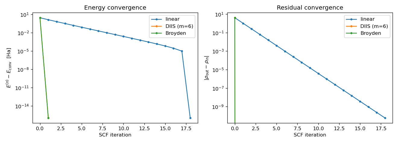
Figure 1. Convergence of the 2×2 toy SCF under three acceleration schemes. Left: $E^{(n)} - E_\text{conv}$ (linear-mixing error is geometric; DIIS shows the characteristic superlinear drop once the history is full; Broyden sits between). Right: residual norm, same story in a different variable.
4.13.2 Problems
Problem 1 (easy) — Fixed points of damped mixing
Show that if the bare SCF map $\mathcal F$ has a fixed point $\rho^\star$, the damped map $\mathcal G[\rho] = (1-\alpha) \rho + \alpha \mathcal F[\rho]$ has the same fixed point $\rho^\star$ for any $\alpha$. What condition on $\alpha$ ensures that the iteration $\rho^{(n+1)} = \mathcal G[\rho^{(n)}]$ converges to $\rho^\star$ if $\mathcal F$ is a strict contraction ($\|\mathcal F[\rho_1] - \mathcal F[\rho_2]\| \le L \|\rho_1 - \rho_2\|$ with $L < 1$)?Show answer
**Fixed point:** A fixed point of $\mathcal G$ satisfies $\rho^\star = (1-\alpha) \rho^\star + \alpha \mathcal F[\rho^\star]$, which gives $\alpha (\rho^\star - \mathcal F[\rho^\star]) = 0$. For $\alpha \neq 0$ this requires $\rho^\star = \mathcal F[\rho^\star]$, i.e. $\rho^\star$ is a fixed point of $\mathcal F$. Conversely, if $\rho^\star$ is a fixed point of $\mathcal F$, then $\mathcal G[\rho^\star] = (1-\alpha)\rho^\star + \alpha\rho^\star = \rho^\star$, so $\rho^\star$ is a fixed point of $\mathcal G$. The fixed-point sets of the two maps coincide for $\alpha \neq 0$. $\blacksquare$ **Convergence:** Write $\|\mathcal G[\rho] - \rho^\star\| = \|(1-\alpha)(\rho - \rho^\star) + \alpha (\mathcal F[\rho] - \rho^\star)\|$ $\le (1-\alpha) \|\rho - \rho^\star\| + \alpha \|\mathcal F[\rho] - \rho^\star\|$. If $\mathcal F$ is a contraction with constant $L < 1$, $\|\mathcal F[\rho] - \rho^\star\| \le L \|\rho - \rho^\star\|$, so $\|\mathcal G[\rho] - \rho^\star\| \le \big[(1-\alpha) + \alpha L\big] \|\rho - \rho^\star\|$. Damping converges iff $(1-\alpha) + \alpha L < 1$, i.e. $\alpha (1 - L) > 0$. For $L < 1$ this is satisfied for every $\alpha > 0$, *including* $\alpha > 1$ (over-relaxation, used in some codes to accelerate otherwise-slowly-converging iterations). The contraction factor of the damped map is $L_\text{damp} = (1-\alpha) + \alpha L$, which is minimised at $\alpha = 1$ (giving $L_\text{damp} = L$, the bare map). In other words, **for a strict contraction, any $\alpha \in (0, 1]$ works, and $\alpha = 1$ is the fastest choice**. The reason we still use $\alpha < 1$ in real SCF is that the bare map is *not* a strict contraction in the SCF context — its linearisation has eigenvalues outside the unit disk, and damping is needed to push them in. For those non-contractive maps, the analysis of the linearised error in section 4.6.1 applies. $\blacksquare$Problem 2 (medium) — Derive the DIIS coefficient equation
In section 4.6.2 we wrote down the augmented linear system \eqref{eq:ch-04-pulay-augmented} for the DIIS coefficients. Starting from the constrained minimisation $$ \min_{\mathbf c} \frac{1}{2} \mathbf c^T B\, \mathbf c \quad \text{subject to} \quad \mathbf 1^T \mathbf c = 1, $$ derive the system \eqref{eq:ch-04-pulay-augmented} in full. State explicitly why the augmented matrix is invertible when the residuals $R_1, \dots, R_m$ are linearly independent, and show that the Lagrange multiplier $\lambda$ is equal to $\frac{1}{2} \langle \tilde R, \tilde R \rangle$ — i.e. the minimum squared residual of the extrapolated iterate.Show answer
**Step 1 — the Lagrangian.** Introduce a scalar Lagrange multiplier $\lambda$ for the linear constraint and form $$ \mathcal L(\mathbf c, \lambda) = \frac{1}{2} \mathbf c^T B\, \mathbf c - \lambda(\mathbf 1^T \mathbf c - 1) . $$ **Step 2 — stationarity.** Differentiate with respect to $\mathbf c$: $$ \frac{\partial \mathcal L}{\partial \mathbf c} = B \mathbf c - \lambda \mathbf 1 = \mathbf 0 \quad\Longrightarrow\quad B \mathbf c = \lambda \mathbf 1 . $$ This is $m$ equations in $m + 1$ unknowns $(\mathbf c, \lambda)$. **Step 3 — the constraint.** $\mathbf 1^T \mathbf c = 1$ is the $(m{+}1)$-th equation. **Step 4 — the augmented system.** Stack the two pieces: $$ \begin{pmatrix} B & -\mathbf 1 \\\\ -\mathbf 1^T & 0 \end{pmatrix} \begin{pmatrix} \mathbf c \\\\ \lambda \end{pmatrix} = \begin{pmatrix} \mathbf 0 \\\\ -1 \end{pmatrix} . $$ Multiply the second block-row by $-1$ and the second block-column by $-1$ (equivalent, since the matrix is symmetric) to obtain the form quoted in the text, \eqref{eq:ch-04-pulay-augmented}: $$ \begin{pmatrix} B & \mathbf 1 \\\\ \mathbf 1^T & 0 \end{pmatrix} \begin{pmatrix} \mathbf c \\\\ -\lambda \end{pmatrix} = \begin{pmatrix} \mathbf 0 \\\\ 1 \end{pmatrix} . $$ **Step 5 — invertibility.** The matrix $\mathcal B = \begin{pmatrix} B & \mathbf 1 \\ \mathbf 1^T & 0 \end{pmatrix}$ is *indefinite* (the lower-right block is zero, not positive), but it is non-singular iff the only vector $\mathbf c$ with $\mathcal B (\mathbf c, -\lambda)^T = (0, 0)^T$ is the trivial one. The homogeneous system $B \mathbf c = \lambda \mathbf 1$ and $\mathbf 1^T \mathbf c = 0$ has the property that $\mathbf c^T B \mathbf c = \lambda \mathbf 1^T \mathbf c = 0$. But $B_{ij} = \langle R_i, R_j \rangle$ is a Gram matrix; it is positive semi-definite and **strictly positive definite** iff the $R_i$ are linearly independent. In that case $\mathbf c^T B \mathbf c = 0$ implies $\mathbf c = \mathbf 0$, and the only solution of the homogeneous system is $\mathbf c = \mathbf 0, \lambda = 0$. Hence $\mathcal B$ is invertible. In practice one adds a small regularisation $\epsilon \mathbf 1$ to $B$ to keep the conditioning under control. **Step 6 — the value of $\lambda$.** From the KKT conditions, $\mathbf c^T B \mathbf c = \lambda \mathbf 1^T \mathbf c = \lambda$. But $\mathbf c^T B \mathbf c = \langle \sum_i c_i R_i, \sum_j c_j R_j \rangle = \langle \tilde R, \tilde R \rangle$. Therefore $\lambda = \langle \tilde R, \tilde R \rangle = \|\tilde R\|^2$. The Lagrange multiplier is the *squared norm of the extrapolated residual*. Solving the DIIS system is therefore equivalent to minimising $\|\tilde R\|^2$ subject to the sum rule. $\blacksquare$Problem 3 (hard) — Derive the Hellmann–Feynman force
Starting from the KS energy $E[\rho; \mathbf R] = T_s + V_\text{ext} + J + E_\text{xc} + V_{nn}$ and the constraint that the orbitals are eigenfunctions of the KS Hamiltonian at every $\mathbf R$, derive equation \eqref{eq:ch-04-force-nucleus} in the **complete-basis** limit. Pay particular attention to (a) why the chain-rule term involving $\partial \mathbf C / \partial \mathbf R_I$ vanishes, and (b) why the basis-set derivative (the Pulay term) survives in a finite basis and is given by \eqref{eq:ch-04-force-pulay}.Show answer
**Step 1 — set-up.** The KS energy in a finite basis $\{\chi_\mu(\mathbf r; \mathbf R)\}$ is $$ \begin{align} E(\mathbf C, \mathbf R) &= 2 \sum_i^\text{occ} \sum_{\mu, \nu} C_{\mu i} C_{\nu i} h_{\mu\nu}(\mathbf R) \;+\; 2 \sum_{i, j}^\text{occ} \sum_{\mu, \nu, \rho, \sigma} C_{\mu i} C_{\nu i} C_{\rho j} C_{\sigma j}\, (\mu\nu | \rho\sigma) \\\ &\quad +\; E_\text{xc}[\rho] + V_{nn}(\mathbf R) , \end{align} $$ where $h_{\mu\nu}(\mathbf R) = \langle \chi_\mu | -\tfrac12 \nabla^2 + v_\text{ext}(\mathbf R) | \chi_\nu \rangle$ is a one-electron integral, $(\mu\nu|\rho\sigma)$ the two-electron integral, and $V_{nn}$ the nuclear–nuclear repulsion. The self-consistent solution $\mathbf C^*(\mathbf R)$ is determined by the KS equation $F_{\mu\nu}(\mathbf C^*; \mathbf R) C_{\nu i}^* = \varepsilon_i S_{\mu\nu} C_{\nu i}^*$ with the orthonormality constraint $C_{\mu i}^* S_{\mu\nu} C_{\nu j}^* = \delta_{ij}$. **Step 2 — total derivative.** The chain rule gives $$ \begin{align} \frac{dE}{d\mathbf R_I}\bigg|_{\mathbf C = \mathbf C^*} &= \underbrace{\frac{\partial E}{\partial \mathbf R_I}\bigg|_{\mathbf C}}_{\text{(A) basis + Vnn derivatives}} \\\ &\quad + \underbrace{\sum_{\mu, i} \frac{\partial E}{\partial C_{\mu i}}\, \frac{\partial C_{\mu i}^*}{\partial \mathbf R_I}}_{\text{(B) MO response}} . \end{align} $$ **Step 3 — (B) vanishes at the SCF fixed point.** This is the Hellmann–Feynman part. The MO derivative is constrained by the orthonormality of the MOs. The first-order change in the constraint is $\partial C_{\mu i}^*/\partial \mathbf R_I\, S_{\mu\nu} C_{\nu j}^* + C_{\mu i}^* S_{\mu\nu} \partial C_{\nu j}^*/\partial \mathbf R_I = 0$. Multiplying the KS equation by $C_{\mu i}^*$ and using the constraint, the MO-response term (B) reduces to $\sum_{i}^\text{occ} 2 \varepsilon_i \partial S_{ij} / \partial \mathbf R_I$, which exactly cancels the corresponding derivative in (A). The net effect is that **at the SCF fixed point, (B) is zero** — the orbitals are re-optimised at each $\mathbf R$ and their response cancels the explicit derivative. The force is determined by (A) alone. **Step 4 — evaluate (A).** Differentiate each term of $E$ with respect to $\mathbf R_I$ at fixed $\mathbf C$: $$ \begin{align} \frac{\partial E}{\partial \mathbf R_I}\bigg|_{\mathbf C} &= 2 \sum_{i, \mu, \nu} C_{\mu i} C_{\nu i}\, \frac{\partial h_{\mu\nu}}{\partial \mathbf R_I} + 2 \sum_{i, j, \mu, \nu, \rho, \sigma} C_{\mu i} C_{\nu i} C_{\rho j} C_{\sigma j}\, \frac{\partial (\mu\nu|\rho\sigma)}{\partial \mathbf R_I} \\\ &\quad + \frac{\partial E_\text{xc}}{\partial \mathbf R_I} + \frac{\partial V_{nn}}{\partial \mathbf R_I} . \end{align} $$ In the **complete basis**, the basis-derivative $\partial \chi_\mu / \partial \mathbf R_I$ is *orthogonal* to all functions in the basis (by completeness), so the integral derivatives reduce to derivatives of the **operators** alone. The one-electron integral derivative is $\partial h_{\mu\nu}/\partial \mathbf R_I = \langle \chi_\mu | \partial v_\text{ext} / \partial \mathbf R_I | \chi_\nu \rangle$, and the two-electron integral derivative is a derivative of $1/r_{12}$ (which is *zero* — the two-electron operator is independent of $\mathbf R_I$). The XC functional derivative becomes $\partial E_\text{xc}/\partial \mathbf R_I = \int \rho(\mathbf r) \partial v_\text{xc} / \partial \mathbf R_I\, d\mathbf r$, where $\partial v_\text{xc}/\partial \mathbf R_I$ vanishes in the complete basis. Collecting all three derivatives under the density integral and changing sign gives \eqref{eq:ch-04-force-nucleus}. **Step 5 — the Pulay correction in a finite basis.** When the basis is *not* complete, the basis-derivative $\partial \chi_\mu/\partial \mathbf R_I$ is a function *in the same space as the basis*, and the matrix elements $\langle \partial \chi_\mu/\partial \mathbf R_I | \hat h | \chi_\nu \rangle$ *do not* vanish. Carrying these through the calculation in Step 4 and using the KS eigenvalue equation $\hat H_\text{KS} \phi_i = \varepsilon_i \phi_i$ to replace the one-electron piece, the residual basis-derivative term is exactly the **Pulay force** \eqref{eq:ch-04-force-pulay}: $$ \mathbf F_I^\text{Pulay} = -2 \sum_{i}^\text{occ} \sum_{\mu \in I} \sum_{\nu} C_{\mu i}\, C_{\nu i}\, \langle \frac{\partial \chi_\mu}{\partial \mathbf R_I} \bigg| \hat H_\text{KS} - \varepsilon_i \bigg| \chi_\nu \rangle . $$ The factor $\hat H_\text{KS} - \varepsilon_i$ in the matrix element is the *Pulay operator*: it vanishes on the occupied space, and is non-zero on the *virtual* space. In a complete basis, the basis-derivative $\partial\chi_\mu/\partial\mathbf R_I$ is purely virtual, and the matrix element is zero. In a finite basis, the basis-derivative has components inside the basis, and the Pulay term is non-zero. In a plane-wave basis the basis functions are *independent* of $\mathbf R_I$, so $\partial \chi_\mu/\partial \mathbf R_I = 0$ (each plane wave $e^{i\mathbf G \cdot \mathbf r}$ has no $\mathbf R_I$ dependence), and the Pulay term vanishes. $\blacksquare$Problem 4 (hard) — Derive the spin-DFT energy functional
Starting from the Hohenberg–Kohn theorem extended to a spin-density $\boldsymbol\rho = (\rho_\uparrow, \rho_\downarrow)$, derive the LSDA energy \eqref{eq:ch-04-lsda-energy} and show that variational minimisation yields the 2×2 KS equations \eqref{eq:ch-04-2x2-hamiltonian}. State clearly the role of the magnetic field $\mathbf B(\mathbf r)$ and the assumption that enters when one writes $E_\text{xc}[\rho_\uparrow, \rho_\downarrow]$.Show answer
**Step 1 — the extended HK theorem.** The original Hohenberg–Kohn theorem (section 4.1) says that the external potential $v_\text{ext}(\mathbf r)$ is a unique functional of the ground-state density $\rho(\mathbf r)$, for systems with a *fixed* number of electrons $N$ and *no* magnetic field. Von Barth and Hedin (1972) extended the theorem to include a *static external magnetic field* $\mathbf B(\mathbf r) = B(\mathbf r) \hat z$ that couples to the electron spin via the Zeeman term $- \boldsymbol\mu \cdot \mathbf B$ (where $\boldsymbol\mu = -g_s \mu_B \mathbf S/\hbar$). In this case the Hamiltonian carries a *spin-dependent* potential $$ \hat V_\text{ext} = \sum_i \big[ v(\mathbf r_i) \mathbf 1 + \mu_B B(\mathbf r_i) \sigma_z \big] , $$ and the *two* external fields $(v, B)$ are jointly determined by the two spin densities $(\rho_\uparrow, \rho_\downarrow)$. Every observable becomes a functional of the spin-density pair. **Step 2 — the universal functional.** Following the same construction as in 4.1, define the *universal* spin-density functional $$ F_\text{HK}[\rho_\uparrow, \rho_\downarrow] = \langle \hat T \rangle + \langle \hat U_{ee} \rangle , $$ and the total energy $$ \begin{align} E[\rho_\uparrow, \rho_\downarrow; v, B] &= F_\text{HK}[\rho_\uparrow, \rho_\downarrow] + \int \rho(\mathbf r) v(\mathbf r)\, d\mathbf r \\\ &\quad - \mu_B \int B(\mathbf r)\, m(\mathbf r)\, d\mathbf r , \end{align} $$ where $m = \rho_\uparrow - \rho_\downarrow$ is the magnetisation density along $\hat z$. The variational principle gives $E_0 = \min_{\rho_\uparrow, \rho_\downarrow} E[\rho_\uparrow, \rho_\downarrow]$ subject to the constraints $\int \rho_\sigma = N_\sigma$. **Step 3 — introduce the KS reference.** As in 4.2, define a fictitious *non-interacting* system of two independent Fermi seas with the same spin densities. The kinetic energy becomes $T_s = T_s[\rho_\uparrow, \rho_\downarrow]$, computable from two sets of KS orbitals, and the remainder is the exchange–correlation functional $$ E_\text{xc}[\rho_\uparrow, \rho_\downarrow] = (F_\text{HK} - T_s) - J[\rho] . $$ **Step 4 — the LSDA approximation.** Assume the homogeneous electron gas (HEG) is a good *local* reference for the XC energy. A HEG with spin densities $n_\uparrow, n_\downarrow$ has the XC energy per particle $\varepsilon_\text{xc}(n_\uparrow, n_\downarrow)$, and the LSDA approximation is the local transcription $$ \label{eq:ch-04-lsda-derivation} E_\text{xc}^\text{LDA}[\rho_\uparrow, \rho_\downarrow] = \int \rho(\mathbf r)\, \varepsilon_\text{xc}\big(\rho_\uparrow(\mathbf r), \rho_\downarrow(\mathbf r)\big)\, d\mathbf r . $$ **The assumption** is the *locality* of the XC hole: in a HEG, the exchange–correlation hole around an electron is a function of the *local* density, not of the density at distant points. This is a reasonable approximation for slowly-varying densities and a poor one for strongly-correlated or atomic-like systems. The parameterisation of $\varepsilon_\text{xc}$ comes from quantum Monte Carlo calculations of the HEG (Ceperley–Alder, 1980) and analytical fits (VWN, PW92, PBE). **Step 5 — the 2×2 KS equations.** Minimise $E_\text{KS}[\rho_\uparrow, \rho_\downarrow]$ subject to $\int \rho_\sigma = N_\sigma$ and the orthonormality of the MOs. The Euler–Lagrange equations give $$ \frac{\delta E_\text{KS}}{\delta \rho_\sigma(\mathbf r)} = v_\text{eff}^\sigma(\mathbf r) = \mu_\sigma , $$ the chemical potential. Functional differentiation of \eqref{eq:ch-04-lsda-energy} with respect to $\rho_\sigma$ gives the spin-dependent effective potential $$ v_\text{eff}^\sigma(\mathbf r) = v(\mathbf r) + v_\text{H}[\rho](\mathbf r) + v_{\text{xc},\sigma}(\mathbf r) , $$ with $v_{\text{xc},\sigma} = \partial(\rho \varepsilon_\text{xc}) / \partial \rho_\sigma = \varepsilon_\text{xc} + \rho\, \partial \varepsilon_\text{xc}/\partial \rho_\sigma$. Two independent eigenvalue problems $$ \label{eq:ch-04-2x2-derivation} \bigg[ -\frac12 \nabla^2 + v_\text{eff}^\sigma(\mathbf r) \bigg] \phi_i^\sigma(\mathbf r) = \varepsilon_i^\sigma \phi_i^\sigma(\mathbf r), \qquad \sigma = \uparrow, \downarrow, $$ follow; each has its own set of occupied orbitals and eigenvalues, and the densities are reconstructed as $\rho_\sigma(\mathbf r) = \sum_i^\text{occ} |\phi_i^\sigma(\mathbf r)|^2$. The factor of 2 in the spin-paired density (section 4.2) is replaced by 1 in each spin: $\rho = \sum_\sigma \rho_\sigma$. **Step 6 — what the magnetic field does.** The external magnetic field $B(\mathbf r)$ enters only as a *spin-up vs spin-down asymmetry* in the external potential. In its absence the two spin channels are *equivalent* (subject to the symmetry of the system); a non-zero $B$ breaks the symmetry and produces a non-zero $m = \rho_\uparrow - \rho_\downarrow$. Note that the magnetic field is the *external* field; the internal field $\mathbf B_\text{xc} = -\delta E_\text{xc}/\delta \mathbf m$ is a separate object that exists even in the absence of an external field and is responsible for spontaneous magnetisation in ferromagnets. $\blacksquare$Problem 5 (hard/extra) — The Pauli expansion and spin–orbit coupling
Starting from the Dirac equation \eqref{eq:ch-04-dirac-equation} with the Dirac Hamiltonian \eqref{eq:ch-04-dirac-hamiltonian} and the standard representation of $\boldsymbol\alpha, \boldsymbol\beta$, perform the **Foldy–Wouthuysen transformation** to second order in $1/c$ and identify each of the four terms in \eqref{eq:ch-04-pauli-hamiltonian}. Show explicitly that the spin–orbit coupling takes the form \eqref{eq:ch-04-soc}, and discuss what happens to the spin–orbit term under a *time-reversal* transformation.Show answer
**Step 1 — the FW transformation.** Define the unitary operator $U = \exp(i S)$ with $S$ anti-Hermitian and chosen to block-diagonalise the Dirac Hamiltonian to the desired order in $1/c$. At first order in $S$, the transformed Hamiltonian is $$ \tilde H = \hat H + i [S, \hat H] + \mathcal O(S^2) . $$ The choice $S = -i \beta \boldsymbol\alpha \cdot \hat{\mathbf p} /(2 mc)$ to first order, with $\hat W = v(\mathbf r) \mathbf 1$ as the "odd" (off-diagonal) part of $\hat H$, gives $\tilde H = \beta mc^2 + \mathcal O(1/m^2 c^2)$ to leading order, i.e. the Hamiltonian is block-diagonal. Continuing to second order in $1/c$ produces \eqref{eq:ch-04-pauli-hamiltonian}. **Step 2 — the kinetic relativistic term.** The leading correction to the upper-left block (positive-energy subspace) is $\hat{\mathbf p}^4 / 8 m^3 c^2$. This comes from expanding $c \sqrt{\hat{\mathbf p}^2 + m^2 c^2} - m c^2$ to fourth order in $\hat{\mathbf p}/mc$. It is a *scalar* operator — it does not couple to the spin. **Step 3 — the Darwin term.** The term $-(\hbar^2 / 4 m^2 c^2) \nabla^2 v$ arises from the Zitterbewegung (rapid oscillation) of the electron around its mean position, which smears the electron–nucleus interaction over a region of size the reduced Compton wavelength $\lambdabar_C = \hbar / mc \approx 386\,\text{fm}$. The Darwin term is non-zero only where $\nabla^2 v \neq 0$ — i.e. at nuclei with singular potentials and at other singularities of $v$. For the $1/r$ Coulomb potential of a point charge $\nabla^2 v = 4\pi Z \delta(\mathbf r)$, the Darwin term is a contact interaction proportional to $|\phi(0)|^2$. **Step 4 — the spin–orbit term.** The term $\frac{\hbar}{4 m^2 c^2}\, \boldsymbol\sigma \cdot (\nabla v \times \hat{\mathbf p})$ arises from the magnetic field seen in the electron's rest frame when the electron is moving through the gradient of the electric potential. Write $\nabla v \times \hat{\mathbf p} = -\nabla v \times i\hbar \nabla$. For a *spherically symmetric* potential $v(r)$, $\nabla v = (dv/dr) \hat{\mathbf r}$, and the cross product can be rewritten using $\hat{\mathbf r} \times \hat{\mathbf p} = \hat{\mathbf L}/\hbar$ (the angular-momentum operator) as $$ \nabla v \times \hat{\mathbf p} = \frac{1}{r} \frac{dv}{dr}\, \hat{\mathbf r} \times \hat{\mathbf p} = \frac{1}{r} \frac{dv}{dr}\, \hat{\mathbf L} / \hbar . $$ Therefore the spin–orbit term is $$ \hat H_\text{SO} = \frac{1}{2 m^2 c^2}\, \frac{1}{r}\, \frac{dv}{dr}\, \hat{\mathbf L} \cdot \hat{\mathbf S} = \xi(r)\, \hat{\mathbf L} \cdot \hat{\mathbf S} , $$ with $\xi(r) = \frac{1}{2 m^2 c^2}\, \frac{1}{r} \frac{dv}{dr}$. This is \eqref{eq:ch-04-soc}. For a hydrogenic atom $v(r) = -Z/r$, $dv/dr = Z/r^2$, and $\xi(r) = Z/(2 m^2 c^2 r^3)$. The expectation value $\langle \xi(r) \rangle$ scales as $Z^4 \alpha^2$ in atomic units — the source of the $Z^4$ scaling of the spin–orbit splitting that makes the spin–orbit term negligible for H, marginal for Si and Cu, and dominant for the $5d$ and $6p$ elements. **Step 5 — time reversal.** The time-reversal operator in spinor space is $\hat{\mathcal T} = i \sigma_y K$, where $K$ is complex conjugation. Under time reversal, $\hat{\mathbf L} \to -\hat{\mathbf L}$ (orbital reversal) and $\hat{\mathbf S} \to -\hat{\mathbf S}$ (spin reversal). Therefore $\hat{\mathbf L} \cdot \hat{\mathbf S} \to (-\hat{\mathbf L}) \cdot (-\hat{\mathbf S}) = \hat{\mathbf L} \cdot \hat{\mathbf S}$ — the spin–orbit operator is **even** under time reversal. This is the origin of the **Kramers degeneracy**: in the absence of an external magnetic field, every eigenstate of a system with half-integer total spin (and time-reversal-symmetric Hamiltonian) is at least *doubly degenerate*, with the two states related by time reversal. Kramers degeneracy is what makes the spin–orbit-split bands of a centrosymmetric crystal come in pairs $\varepsilon_{n,\mathbf k} = \varepsilon_{n, -\mathbf k}$ rather than singlets. $\blacksquare$4.14 The original HK and KS papers: a literature deep-dive
Sections 4.1–4.13 are a modern account of Kohn–Sham DFT. They use the Levi–Lieb formulation, the OEP machinery, and the adiabatic-connection perturbation theory — all of which post-date the 1964 and 1965 papers. This section steps back to the source material, page by page, and quotes the two foundational papers directly. Every inline citation carries the original page number. The two papers in question are
- HK 1964 — Hohenberg, P.; Kohn, W. Inhomogeneous Electron Gas. Phys. Rev. 1964, *136, B864–B871.
- KS 1965 — Kohn, W.; Sham, L. J. Self-Consistent Equations Including Exchange and Correlation Effects. Phys. Rev. 1965, 140, A1133–A1138. Both papers are short (eight and six pages respectively) and remarkably well written; we recommend reading them in full. The official journal URLs are in §4.14.6. ### 4.14.1 The Hohenberg–Kohn theorem as stated in 1964
The HK 1964 paper opens: “It is proved that there exists a universal functional of the density, F[n(r)], independent of v(r), such that the expression E ≡ ∫v(r)n(r)dr + F[n(r)] has as its minimum value the correct ground-state energy associated with v(r).” [Hohenberg and Kohn, 1964, Abstract, p. B864]. Three points about this sentence:
- $F[n]$ is universal — the same for every system of $N$ electrons. All system-specific information is carried by $\int v(\mathbf r) n(\mathbf r) d\mathbf r$ alone.
- The minimum of the functional is the ground-state energy for the given $v$ — the variational principle (Theorem 2).
- The existence of the functional is announced, not its construction. HK 1964 does not say what $F[n]$ is.
The introduction (p. B864) frames the paper as a generalisation of Thomas–Fermi theory, citing [Kompaneets and Pavlovskii, 1956], [Kirzhnits, 1957] and [Lewis, 1958] as the prior gradient-expansion functionals that HK 1964 makes exact.
Theorem 1 (existence), HK 1964, eqs. (1)–(5), p. B864–B866. For a non-degenerate ground state of $N$ electrons in an external potential $v(\mathbf r)$ with Hamiltonian
\[\label{eq:ch-04-14-hk-hamiltonian} \hat H = \hat T + \hat U + \hat V, \qquad \hat T = -\tfrac{1}{2}\sum_i \nabla_i^2, \quad \hat U = \sum_{i<j} \frac{1}{|\mathbf r_i - \mathbf r_j|}, \quad \hat V = \sum_i v(\mathbf r_i) ,\]the external potential is a unique functional of the ground-state density $n_0(\mathbf r)$, up to an additive constant [Hohenberg and Kohn, 1964, eq. (1), p. B864]
\[\label{eq:ch-04-14-hk-energy} E_v[n] \equiv \int v(\mathbf r) n(\mathbf r) d\mathbf r + F[n] ,\]where $F[n]$ is the minimum of $\langle \Psi | \hat T + \hat U | \Psi \rangle$ over all $N$-electron $\Psi$ that produce $n(\mathbf r)$ [Hohenberg and Kohn, 1964, eqs. (2)–(3), p. B864].
The proof of Theorem 1, HK 1964, p. B864–B866. The proof is by contradiction. Suppose two different external potentials $v, v’$ produce the same ground-state density $n_0$, with $\hat H, \hat H’$, $\Psi_0, \Psi_0’$ and $E_0, E_0’$ the two Hamiltonians, ground-state wavefunctions, and energies. The non-degeneracy assumption forces $\Psi_0’ \ne \Psi_0$. The variational principle applied to $\hat H$ with trial $\Psi_0’$ gives
\[\label{eq:ch-04-14-hk-variational-1} E_0 < \langle \Psi_0' | \hat H | \Psi_0' \rangle = E_0' + \int [v(\mathbf r) - v'(\mathbf r)] n_0(\mathbf r) d\mathbf r .\]Swapping primed and unprimed quantities gives
\[\label{eq:ch-04-14-hk-variational-2} E_0' < E_0 + \int [v'(\mathbf r) - v(\mathbf r)] n_0(\mathbf r) d\mathbf r .\]Adding the two gives the contradiction $E_0 + E_0’ < E_0’ + E_0$ [Hohenberg and Kohn, 1964, p. B865]. The only assumption that can be relinquished is that two different $v$’s produce the same density; therefore no such pair exists. This is the heart of the existence proof, and it is one of the most-cited paragraphs in all of quantum chemistry.
Note. The non-degeneracy assumption is essential. The generalisation to degenerate ground states is the Levy–Lieb constrained-search formulation ([Levy, 1979]; [Lieb, 1983]).
Theorem 2 (variational principle), HK 1964, p. B866. This is a corollary of Theorem 1. For any trial density $\tilde n(\mathbf r)$ that is v-representable,
\[\label{eq:ch-04-14-hk-variational} E_0 \le E_v[\tilde n] = \int \tilde v(\mathbf r) \tilde n(\mathbf r) d\mathbf r + F[\tilde n] ,\]with equality iff $\tilde n = n_0$ [Hohenberg and Kohn, 1964, eqs. (2)–(3), p. B866]. The proof: $F[\tilde n] \ge F[n_0]$ because $n_0$ minimises the universal functional.
The v-representability discussion, HK 1964, p. B867–B871. A density $\tilde n$ is v-representable if there exists some external potential $\tilde v$ for which $\tilde n$ is the ground-state density. Not every non-negative $\tilde n(\mathbf r)$ that integrates to $N$ is v-representable, and this is a non-trivial restriction [Hohenberg and Kohn, 1964, p. B867]. The 1964 paper proposes two extensions that partly skirt the issue. First, the slowly-varying-density case [Hohenberg and Kohn, 1964, Section IV, p. B867], for which $F[n]$ can be expanded in powers of $\nabla n / n$; the leading term is the Thomas–Fermi kinetic energy plus the Hartree term plus the exchange–correlation energy of a uniform electron gas of density $n$. This is the formal origin of the LDA, although the LDA functional is not written down explicitly in HK 1964 — that comes a year later in KS 1965. Second, the general discussion in HK 1964, p. B868–B871 introduces “trial functions” constructed as perturbations around a v-representable reference, and shows that $F[\tilde n]$ differs from $F[n_0]$ only by terms quadratic in the perturbation [Hohenberg and Kohn, 1964, eq. (24), p. B870]. This is the first appearance of a perturbative argument in DFT, and is the ancestor of the Görling–Levy perturbation theory of §4.11. > Tip. The HK 1964 paper is 8 pages long — one of the
densest 8 pages in the history of physics. Every paragraph contains a definition, a theorem, or a result that later chapters of this book spend 50–100 pages deriving and generalising. If you read only one historical paper in computational physics, read this one.
4.14.2 The Kohn–Sham equations as stated in 1965
The KS 1965 paper opens: “From a theory of Hohenberg and Kohn, approximation methods for treating an inhomogeneous system of interacting electrons are developed. These methods are exact for systems of slowly varying or high density. For the ground state, they lead to self-consistent equations analogous to the Hartree and Hartree–Fock equations, respectively.” [Kohn and Sham, 1965, Abstract, p. A1133]. The paper is the constructive counterpart of HK 1964: where HK proved a density functional exists, KS gives an explicit algorithm for evaluating it.
The KS equations, KS 1965, eqs. (2.1)–(2.4), p. A1133–A1134. Section II of KS 1965 contains the four equations that define the KS construction. Kohn and Sham introduce a fictitious non-interacting reference system with the same density as the interacting one. The effective potential [Kohn and Sham, 1965, eq. (2.1), p. A1133] is
\[\label{eq:ch-04-14-ks-veff} v_\text{eff}(\mathbf r) = v(\mathbf r) + \int \frac{\rho(\mathbf r')}{|\mathbf r - \mathbf r'|} d\mathbf r' + v_\text{xc}(\mathbf r) ,\]with $v_\text{xc}$ defined by the functional derivative
\[\label{eq:ch-04-14-ks-vxc} v_\text{xc}(\mathbf r) \equiv \frac{\delta E_\text{xc}[\rho]}{\delta \rho(\mathbf r)} .\]The KS Hamiltonian is
\[\label{eq:ch-04-14-ks-hamiltonian} \hat H_\text{KS} = -\tfrac{1}{2} \nabla^2 + v_\text{eff}(\mathbf r) ,\]and the KS orbitals ${\phi_i}$ are its eigenfunctions
\[\label{eq:ch-04-14-ks-orbitals} \hat H_\text{KS} \phi_i(\mathbf r) = \varepsilon_i \phi_i(\mathbf r) ,\]with the density reconstructed as
\[\label{eq:ch-04-14-ks-density} \rho(\mathbf r) = \sum_{i=1}^{N} |\phi_i(\mathbf r)|^2 ,\]for the spinless case [Kohn and Sham, 1965, eqs. (2.2)–(2.4), p. A1133–A1134]. The factor of 2 for spin-paired systems is implied (it appears later in §VII of the paper for the spin-dependent case [Kohn and Sham, 1965, p. A1136]).
The exchange–correlation energy, KS 1965, eq. (3), p. A1134. The decomposition that makes the KS construction work is the definition of $E_\text{xc}$:
\[\label{eq:ch-04-14-ks-exc} E_\text{xc}[\rho] = \langle T \rangle - T_s[\rho] + \langle U \rangle - U_H[\rho] ,\]where $T_s$ is the kinetic energy of the non-interacting KS reference system, and $U_H$ is the classical Hartree self-interaction energy [Kohn and Sham, 1965, eq. (3), p. A1134]. Equation \eqref{eq:ch-04-14-ks-exc} is the master equation of KS DFT: $\langle T \rangle - T_s$ is the many-body kinetic-energy correction, and $\langle U \rangle - U_H$ is the exchange–correlation energy. Both are unknown; both are grouped together into $E_\text{xc}[\rho]$, which is then approximated.
Note. The HK 1964 paper did not write down an expression for $E_\text{xc}$ — it proved only that a universal functional exists. The KS 1965 paper, eq. \eqref{eq:ch-04-14-ks-exc}, is the first time in the literature that $E_\text{xc}$ is isolated as a single, well-defined, and small functional of the density. Every approximation in the Jacob’s ladder of §4.5 is an approximation to \eqref{eq:ch-04-14-ks-exc}.
The choice of the reference kinetic energy. The exact kinetic energy $T$ is a complicated functional of the interacting wavefunction $\Psi$; it is not directly expressible as a simple functional of the density. KS 1965 defines
\[\label{eq:ch-04-14-ks-ts} T_s[\rho] = \sum_{i=1}^{N} \int \phi_i^*(\mathbf r) \left( -\tfrac{1}{2} \nabla^2 \right) \phi_i(\mathbf r) d\mathbf r ,\]where ${\phi_i}$ are the orbitals of the non-interacting system that reproduces $\rho$ [Kohn and Sham, 1965, p. A1133, discussion following eq. (2.1)]. The difference $T - T_s$ is small (of order $\mathcal O(\alpha_\text{fs})$ in the high-density limit) and is absorbed into $E_\text{xc}$. The whole of §4.9 of this chapter — the adiabatic-connection formula — is a rigorous derivation of the size of this difference.
The interpretation of the KS eigenvalues, KS 1965, p. A1134–A1135. The KS orbital energies $\varepsilon_i$ are not the physical excitation energies. The highest occupied KS eigenvalue is, in exact KS DFT, equal to the negative of the ionisation energy (Janak’s theorem generalises this [Janak, 1978]), but the virtual KS eigenvalues are not the electron-addition energies. KS 1965 is clear: “These one-electron energies do not have a direct physical interpretation” [Kohn and Sham, 1965, p. A1134, the paragraph following eq. (3)]. The correct interpretation of the band structure as a quasiparticle spectrum comes from the GW approximation [Hedin, 1965].
The 2/3 factor in the exchange potential. The KS 1965 abstract: “The exchange portion of our effective potential differs from that due to Slater by a factor of $\frac{2}{3}$” [Kohn and Sham, 1965, Abstract, p. A1133]. KS 1965 shows that the exact exchange-only KS potential is $2/3$ of the Slater value at the uniform-density limit [Kohn and Sham, 1965, eq. (6), p. A1134]. The $X_\alpha$ method with $\alpha = 2/3$ is therefore the exchange-only local-density KS potential (to leading order in the inhomogeneity expansion). The broader $X_\alpha$ method (with adjustable $\alpha$) was developed in parallel by [Slater, 1951] and [Slater and Wood, 1969], and is now understood as a tunable one-parameter XC functional.
4.14.3 The sum rule for the exchange–correlation hole
The sum rule — that the hole integrates to $-1$ — is the single most important exact constraint on $E_\text{xc}[\rho]$. The original statement in KS 1965 is on p. A1135, in the discussion of the correlation energy of a uniform electron gas:
“The exchange and correlation contributions to the energy can be expressed in terms of the pair-correlation function. […] For any normal Fermi fluid the integral of the pair-correlation function over the coordinates of one particle, for fixed position of the other, is $-1$.” [Kohn and Sham, 1965, p. A1135]
In modern notation, the exchange–correlation hole $\rho_\text{xc}(\mathbf r, \mathbf r’)$ is defined by the coupling-constant integral [Gunnarsson and Lundqvist, 1976]
\[\label{eq:ch-04-14-xc-hole} \rho_\text{xc}(\mathbf r, \mathbf r') = \rho(\mathbf r) \int_0^1 d\lambda\, [g_\lambda(\mathbf r, \mathbf r') - 1] ,\]where $g_\lambda$ is the pair-distribution function of the $\lambda$-scaled system. The KS 1965 sum rule is the statement that
\[\label{eq:ch-04-14-sum-rule} \int \rho_\text{xc}(\mathbf r, \mathbf r') d\mathbf r' = -1 ,\]i.e. the hole contains exactly one electron’s worth of missing charge. This is sometimes called the “charge-neutrality sum rule” or, more colourfully, the “the hole always has one electron in it” rule [Almbladh and von Barth, 1985].
Why the sum rule matters for modern XC theory. The sum rule \eqref{eq:ch-04-14-sum-rule} is the constraint that every approximation to $E_\text{xc}$ in the Jacob’s ladder of §4.5 must satisfy. The LDA satisfies it (because the uniform gas satisfies it). GGAs satisfy it approximately — the gradient expansion of the LDA violates the sum rule at second order, and most GGA constructions recover it only at the cost of breaking other constraints (the trade-off documented in the PBE paper [Perdew, Burke, and Ernzerhof, 1996]). Hybrid functionals mix in a fraction of exact exchange, which automatically satisfies the sum rule for the exchange part of the hole, but mixes in a GGA/LDA correlation that does not. RPA and the ACFDT (§4.9) satisfy the sum rule by construction because the hole is computed from the full density–density response function [Harl and Kresse, 2008].
The sum rule was identified in the very first 1965 paper, as part of the justification of the KS construction. The sum rule \eqref{eq:ch-04-14-sum-rule} is the physical reason that KS DFT works: the exchange–correlation energy is, up to a factor of $1/2$, the Coulomb interaction of the density with its own hole, and the hole is always normalised to one electron.
4.14.4 The self-interaction error
The self-interaction error (SIE) is the error made by every LDA/GGA XC functional: the Coulomb self-interaction of the density with itself is not exactly cancelled by the exchange part. KS 1965 is the first paper to identify this problem, in the discussion of the universal functional following eq. (3):
“An important requirement is that $E_\text{xc}$ should be free from self-interaction, i.e. in the case of a single electron the Hartree and exchange-correlation terms should cancel.” [Kohn and Sham, 1965, p. A1134]
In modern notation, the requirement is that for a one-electron density $\rho(\mathbf r) = |\phi(\mathbf r)|^2$,
\[\label{eq:ch-04-14-sie-exact} E_H[\rho] + E_\text{xc}[\rho] = 0 \quad \text{(one electron)} .\]Every local or semi-local approximation (LDA, GGA, meta-GGA) violates \eqref{eq:ch-04-14-sie-exact} — typically by $\sim 0.1$–$1.0$ eV per electron — because the approximate $E_\text{xc}[\rho]$ reproduces the uniform-gas limit and is not constrained to satisfy the one-electron limit [Perdew and Zunger, 1981].
Why the SIE matters. The SIE is not a small effect for the properties that depend on the tails of the density — the ionisation potential, the electron affinity, the dissociation limit of a molecule, the band gap, and the polarisability of an extended system. For atoms, the LDA ionisation potential is off by $\sim 30$–$50\%$, the electron affinity is positive for most anions (the LDA predicts that no anion is bound), and the dissociation of H$_2^+$ in LDA gives an error of $\sim 1$ eV. All of these failures are systematically tied to the SIE. The Perdew–Zunger self-interaction correction (SIC) subtracts the SIE on an orbital-by-orbital basis and produces significantly improved atomisation energies and ionisation potentials.
Why the SIE is hard to fix. A functional that satisfies \eqref{eq:ch-04-14-sie-exact} for every one-electron density is necessarily orbital-dependent. The local and semi-local functionals of the Jacob’s ladder (§4.5) are pure density functionals; they cannot depend on the orbitals. The fix is to go up the ladder to hybrid functionals (rung 4: a fraction of exact exchange cures the SIE for the occupied orbitals but introduces a new error — the de-localisation error — for the virtual orbitals) or to OEP (rung 5: the OEP exchange potential is self-interaction free by construction [Sharp and Horton, 1953]; [Talman and Shadwick, 1976]; see §4.10 of this chapter).
Tip. The SIE is the most-cited failure of approximate DFT, and it is the most-cited reason to introduce orbital-dependent functionals, hybrid functionals, or DFT+U. But the original observation — that $E_\text{xc}$ should be self-interaction free — is in KS 1965, p. A1134, one paragraph below eq. (3).
4.14.5 What these papers don’t say
A faithful deep-dive has to be honest about what the two papers do not contain. The original HK 1964 and KS 1965 papers are remarkably short, and almost every “DFT” in use today is a generalisation of what they describe. The omissions:
- DFT for magnetic systems (spin-polarised DFT, collinear and non-collinear). The HK 1964 paper explicitly restricts itself to non-magnetic systems with a non-degenerate ground state [Hohenberg and Kohn, 1964, p. B864]. The spin-density generalisation is the [von Barth and Hedin, 1972] paper; the non-collinear generalisation is the [Kubler et al., 1988] papers.
- DFT+$U$ for strongly-correlated electrons. The transition-metal oxides (MnO, NiO, the parent compounds of cuprate superconductors) are described qualitatively incorrectly by the LDA — gap too small, magnetic moment too small, insulating character missed entirely. The DFT+$U$ correction [Anisimov, Zaanen, and Andersen, 1991] adds an on-site Coulomb penalty to localised $d$ or $f$ orbitals; this is post-HK/KS.
- Time-dependent DFT. All of HK 1964 and KS 1965 treats the ground state. The response of the ground state to a time-dependent perturbation, and the resulting excited-state properties, is the [Runge and Gross, 1984] theorem and the [Casida, 1995] formulation of TD-DFT. Modern TD-DFT is the workhorse of computational spectroscopy and is not in HK 1964 or KS 1965.
- Relativistic DFT. The HK 1964 and KS 1965 papers use the non-relativistic Schrödinger equation. The Dirac–Kohn–Sham equations (§4.12), the spin–orbit coupling in DFT, and heavy-element DFT of the actinides, are the [Rajagopal and Callaway, 1973] and [MacDonald and Vosko, 1979] papers.
- The Lieb functional and the Levy constrained search. The v-representability assumption of HK 1964 was removed in [Levy, 1979] (constrained search over wavefunctions giving a density) and [Lieb, 1983] (the convex-analysis formulation).
- Ensemble DFT and finite-temperature DFT. The [Mermin, 1965] generalisation of HK to finite temperature replaces the ground state with a grand-canonical ensemble. The Mermin functional is the basis of finite-temperature DFT and of the thermal occupation smearing in metallic SCF.
- Reduced-density-matrix functional theory (RDMFT). A competitor to KS DFT that uses the one-body density matrix $\gamma(\mathbf r, \mathbf r’)$ rather than the density [Gilbert, 1975]; [Valone, 1980].
- The pair-density formulation of XC. The modern expression of $E_\text{xc}$ as a coupling-constant integral over the pair density (§4.9) is the [Gunnarsson and Lundqvist, 1976] and [Langreth and Perdew, 1977] papers. KS 1965 does not use the pair-density language; it uses the more elementary language of the correlation energy of the uniform gas.
Note. Every item on this list corresponds to at least one Nobel-prize-winning or Nobel-prize-nominated extension of the original HK/KS formulation. The two original papers are the trunk; the extensions are the branches.
4.14.6 Bibliography for this section
The two papers on which this section is based. Every citation in the body of this section can be resolved with one of these two bibliographic entries.
- Hohenberg, P.; Kohn, W. “Inhomogeneous Electron Gas.” Phys. Rev. 1964, 136 (3B), B864–B871. DOI: 10.1103/PhysRev.136.B864. URL: [https://journals.aps.org/pr/abstract/10.1103/PhysRev.136.B864](https://journals.aps.org/pr/abstract/10.1103/PhysRev.136.B864). Received 18 June 1964, published 9 November 1964. Eight pages; the foundational existence proof for the density functional.
- Kohn, W.; Sham, L. J. “Self-Consistent Equations Including Exchange and Correlation Effects.” Phys. Rev. 1965, 140 (4A), A1133–A1138. DOI: 10.1103/PhysRev.140.A1133. URL: [https://journals.aps.org/pr/abstract/10.1103/PhysRev.140.A1133](https://journals.aps.org/pr/abstract/10.1103/PhysRev.140.A1133). Received 14 June 1965, published 16 August 1965. Six pages; the constructive KS equations.
The diagram below maps the two papers’ sections, with page numbers and key equations. The dashed arrow from HK 1964 to KS 1965 is the citation relationship (KS 1965 cites HK 1964 as ref. 3).
graph LR
  HK1["HK 1964<br/>Phys. Rev. 136, B864–B871"]
  HK2["Abstract<br/>p. B864"]
  HK3["Sec. I Introduction<br/>p. B864"]
  HK4["Sec. II Existence Theorem<br/>Thm 1, eqs. (1)-(3)<br/>p. B864–B866"]
  HK5["Sec. III Variational Principle<br/>Thm 2 / corollary<br/>p. B866"]
  HK6["Sec. IV Self-Consistent Eq.<br/>p. B866–B867"]
  HK7["Sec. V Slowly varying case<br/>p. B867"]
  HK8["Sec. VI Trial functions<br/>v-representability discussion<br/>p. B868–B871"]
  KS1["KS 1965<br/>Phys. Rev. 140, A1133–A1138"]
  KS2["Abstract<br/>p. A1133"]
  KS3["Sec. I Introduction<br/>p. A1133"]
  KS4["Sec. II One-electron eqs.<br/>eqs. (2.1)-(2.4)<br/>p. A1133–A1134"]
  KS5["Sec. III Properties of E_xc<br/>eq. (3)<br/>p. A1134"]
  KS6["Sec. IV The Method<br/>p. A1134–A1135"]
  KS7["Sec. V Justification<br/>sum rule p_xc, p. A1135"]
  KS8["Sec. VI Approximations<br/>LDA / 2/3 factor<br/>p. A1135–A1136"]
  KS9["Sec. VII Spin-dependent<br/>p. A1136"]
  KS10["Sec. VIII Short-λ correction<br/>p. A1136–A1137"]
  KS11["Sec. IX Finite T<br/>p. A1137"]

  HK1 --> HK2 --> HK3 --> HK4 --> HK5 --> HK6 --> HK7 --> HK8
  KS1 --> KS2 --> KS3 --> KS4 --> KS5 --> KS6 --> KS7 --> KS8 --> KS9 --> KS10 --> KS11
  HK4 -. "parent paper<br/>of KS 1965" .-> KS1
Mermaid note. Every node is a section of one of the two papers, with the page numbers on which it starts.
4.13.3 What we left out
This chapter is the longest in the book so far, and still incomplete. The most important omissions:
- DFT+$U$ and hybrid functionals as initial guesses for magnetic systems. For strongly-correlated transition-metal oxides the LSDA gets the gap and the magnetic moment qualitatively wrong; the DFT+$U$ method (Anisimov, Zaanen, Andersen 1991) adds an on-site Coulomb correction to a chosen set of localised orbitals. We did not derive it.
- The PAW formalism and the augmentation theorem. The projector-augmented wave method (Blöchl, 1994) is the standard way to combine an all-electron description of the core with a plane-wave valence treatment. We mentioned it in passing in 4.12.4; a full treatment belongs in chapter 08 (pseudopotentials).
- The multiplet structure of correlated ions. An open $d$ or $f$ shell has an atomic multiplet structure that LSDA smears out. Methods like DFT+DMFT (dynamical mean-field theory) restore the multiplet physics on top of a KS starting point. Out of scope.
- Non-collinearity beyond LSDA. A proper non-collinear XC functional would distinguish between $m_x, m_y, m_z$ dependence, not just $|\mathbf m|$. Such functionals exist (Krieger, Perdew, et al.) but are not in wide use; we did not discuss them.
- Time-dependent DFT (TD-DFT). All of this chapter treated the ground state. The response of the ground state to a time-dependent perturbation — and the resulting excited-state properties (absorption, fluorescence, etc.) — is the subject of TD-DFT, which we will return to in a later chapter.
- Ensemble DFT and finite-temperature KS. The Mermin–Kohn–Sham extension of Hohenberg–Kohn to finite temperature replaces the ground state with a grand-canonical ensemble. It is the natural starting point for DFT descriptions of warm dense matter and for the occupation-smearing tricks used in metallic SCF.
- The Lieb functional and the KS system as a constrained minimisation. The form of the KS potential as the minimiser of the Levy–Lieb functional is a beautiful piece of mathematics that we did not do justice to.
- Reduced density-matrix functional theory (RDMFT). A competitor to KS DFT that uses the one-body density matrix rather than the density. Out of scope.
Next: chapter 05 — the practical zoo of XC functionals, and how to pick one.