Chapter 13 — DFT+U & beyond
Standard Kohn–Sham DFT works because the exchange–correlation functional gets the total energy almost right. Almost. For materials with partially-filled $d$ and $f$ shells — the transition-metal oxides, the rare earths, the actinides, the high-$T_c$ cuprates — “almost” is not enough. This chapter is about the corrections that fix it, and the methods that are enough.
By the end of chapter 05 we had the full Kohn–Sham machinery: a fictitious non-interacting reference system that reproduces the interacting density, a self-consistent loop, and a Jacobian’s ladder of exchange–correlation functionals — LDA, GGA, meta-GGA, hybrid. For most of chemistry and materials science, the local and semi-local rungs of that ladder are good enough; even the hybrid rung (PBE0, B3LYP) gets the thermochemistry of organic molecules within $\sim 0.2\,\text{eV}$. The exceptions are the materials where the most interesting physics lives in a few partially-filled orbitals — the $3d$ shell of a transition metal, the $4f$ shell of a lanthanide, the $5f$ shell of an actinide. There, the LDA and GGA make characteristic mistakes: a Mott insulator comes out metallic, a band gap is underestimated by a factor of two, and a satellite peak in the photoemission spectrum is missing entirely. This chapter is the “where the rubber meets the road” chapter for correlated materials. We will, in order: state the qualitative failure (§ 13.1); introduce the Hubbard model that contains the missing physics (§ 13.2.2); derive the DFT+U correction that adds Hubbard physics to LDA (§§ 13.2.3–13.2.4); survey the systematic beyond-DFT approaches — range-separated hybrid functionals (§ 13.2.5), the GW self-energy (§ 13.2.6), and dynamical mean-field theory (§ 13.2.7); close with the side-by-side comparison (§ 13.2.8), a worked exact-diagonalisation example on the 4-site Hubbard model (§ 13.5), three graded problems (§ 13.6), and an honest list of omissions (§ 13.10).
Reading note. This chapter assumes chapters 04 (Kohn–Sham DFT) and 05 (XC functionals). The reading of chapter 13 is optional for the rest of the chapters in this series — chapters 06–12 do not use it. It is, however, the natural starting point for any reader who plans to compute the properties of transition-metal oxides, rare-earth compounds, or any other material with partially-filled $d$ or $f$ shells.
13.1 The claim
The headline is a one-line statement of where standard DFT fails, what fixes it, and what each fix costs.
Claim. Standard Kohn–Sham DFT with a local or semi-local XC functional systematically fails for materials with partially-filled $d$ or $f$ shells: Mott insulators are predicted metallic, band gaps are underestimated by $\sim 50\%$, and the satellite peaks of the spectral function are absent. The DFT+U correction restores the local physics at the price of an empirical Hubbard $U$ parameter. The systematic, parameter-free many-body methods — screened hybrid functionals, the GW self-energy, and dynamical mean-field theory — capture the same physics at a sharply higher computational cost.
The claim is compact. The rest of the chapter unpacks it. The point of entry is the atomic limit of a partially-filled shell. An isolated Mn$^{2+}$ ion ($3d^5$, half-filled, $S = 5/2$) has an integer number of $d$ electrons in the Hund’s-rule ground state, and a gap of $\sim 5\,\text{eV}$ to the first excited state. In MnO (the rock-salt antiferromagnet) the same $d$ electrons are localised, the same gap is present, and the material is a transparent insulator with a $\sim 4\,\text{eV}$ gap. The local physics has not changed between the ion and the solid; what has changed is the competition between the on-site Coulomb repulsion $U$ that wants to localise the electrons and the inter-site hopping $t$ that wants to delocalise them. When $U \gg t$, the electrons stay local and the material is a Mott insulator; when $t \gg U$, the electrons delocalise and the material is a band metal. The phase boundary is the Mott transition, and it is not a phase transition of the LDA — the standard XC functional does not know about $U$ at all. The result is the characteristic failure:
\[\label{eq:ch-13-claim} \boxed{\; \Delta_\text{exp} \;\approx\; 2 \Delta_\text{LDA} \quad \text{and} \quad \Sigma_\text{sat}(\omega) \Big|_{\text{LDA}} \equiv 0 , \quad \text{for } 3d\text{ oxides and } 4f\text{ compounds.} \;}\]The first equality says that the LDA band gap is roughly half the experimental gap; the second says that the LDA spectral function $A(\omega)$ has no satellite (the $\sim 6\,\text{eV}$ lower-Hubbard-band peak of Ni is entirely missing). The Hubbard $U$ enters as the only parameter that has to be supplied by the user; once it is in place, the rest of the machinery — the localised orbital, the occupation matrix, the double-counting correction — is fixed by the formalism.
The reader who wants a quick summary of the methods covered in this chapter should jump straight to § 13.2.8 and return. The reader who wants to see why the LDA fails, and how each correction fixes it, should read the chapter in order.
13.2 The derivation
This section contains the substantive material: the failure mode of LDA, the Hubbard model, the DFT+U correction, the choice of $U$, the hybrid-functional route, the GW self-energy, and the DMFT outlook.
13.2.1 The failure of LDA for Mott insulators
The diagnostic numbers are old. Table 1 collects the experimental band gaps of the late-$3d$ transition-metal monoxides (MnO, FeO, CoO, NiO) alongside the LDA predictions and the GGA+U values with a representative $U$ on the metal $3d$ shell. The LDA underestimates the gap by a factor of 2; the underestimation is systematic, not statistical, and it correlates with the number of $d$ electrons.
Table 1. Band gaps of the late-$3d$ monoxides (eV). The columns compare experiment, LDA, GGA (PBE), GGA+U with $U_\text{eff} = U - J \sim 4$–$5\,\text{eV}$, and HSE06 hybrid. All values are for the antiferromagnetic ground state. The LDA/GGA systematic underestimation is the signature of the missing Mott physics.
| Compound | Configuration | $E_g^\text{exp}$ | $E_g^\text{LDA}$ | $E_g^\text{PBE}$ | $E_g^\text{GGA+U}$ | $E_g^\text{HSE06}$ |
|---|---|---|---|---|---|---|
| MnO | $3d^5$ | 3.9 – 4.1 | 0.8 – 1.0 | 0.9 – 1.2 | 3.5 – 3.9 | 3.6 – 4.0 |
| FeO | $3d^6$ | 2.4 | 0.0 (metal!) | 0.0 (metal!) | 2.0 – 2.4 | 2.3 – 2.6 |
| CoO | $3d^7$ | 2.5 – 2.8 | 0.0 (metal!) | 0.0 (metal!) | 2.3 – 2.7 | 2.5 – 2.9 |
| NiO | $3d^8$ | 4.0 – 4.5 | 0.4 – 0.6 | 0.5 – 0.8 | 3.3 – 4.0 | 4.0 – 4.5 |
(Sources: experiment — van Elp et al., Phys. Rev. B 44, 6090 (1991); LDA/PBE — standard plane-wave calculations with a $30$–$50\,\text{Ry}$ cutoff; GGA+U — Dudarev et al., Phys. Rev. B 57, 1505 (1998); HSE06 — Heyd, Scuseria, Ernzerhof, J. Chem. Phys. 118, 8207 (2003).)
The quantitative failure of LDA is bad enough. The qualitative failure is worse: FeO and CoO come out metallic — the wrong phase, the wrong physics, the wrong answer to the question “is this material a conductor?”. The error has a name and a cause.
Cause. The LDA XC potential $v_\text{xc}(\mathbf r)$ is a local functional of the density. The self-interaction correction that is missing for a localised $d$ electron is a non-local effect — it depends on the occupancy of the $d$ orbital on this atom, not on the density at $\mathbf r$. The LDA cannot simulate it because it does not know which density belongs to which orbital. In the language of the Hubbard model, the LDA XC potential acts on the $d$ electron as if $U_\text{eff} = 0$ — it cannot penalise the double occupancy of the $d$ shell. The result is that the $d$ band is too wide (because each $d$ electron sees the full hybridisation with its neighbours) and the gap is too small (or vanishing).
The spectral function is the cleanest way to see the failure. In a one-particle picture, the photoemission spectrum at energy $\omega$ is
\[\label{eq:ch-13-spectral} A(\mathbf k, \omega) \;=\; \sum_n \Bigl| \langle \phi_n | \psi_{\mathbf k} \rangle \Bigr|^2\, \delta(\omega - \varepsilon_n) ,\]a sum of delta functions at the quasi-particle (QP) energies. In a Mott insulator, the many-body spectral function is qualitatively different. The ground state of the atom has integer $d$-occupancy; removing one electron from the occupied $d$ band costs an energy $\sim -(\varepsilon_d + U)$ (the lower Hubbard band), and removing it from the unoccupied $d$ band costs $\sim -\varepsilon_d$ (the upper Hubbard band). The splitting between the two is the Hubbard $U$:
\[\label{eq:ch-13-hubbard-split} \Delta_\text{Hubbard} \;=\; \varepsilon_{d}^{UHB} - \varepsilon_{d}^{LHB} \;\approx\; U - W ,\]where $W$ is the $d$-band width. The LDA misses the splitting entirely: it puts the $d$ band in one place, at the bare $\varepsilon_d$, and the spectral weight that should be in the lower Hubbard band is redistributed into a metallic quasi-particle peak at $\varepsilon_d$. The satellite at $\sim -6\,\text{eV}$ in Ni (the famous “6-eV satellite”) is the lower Hubbard band, and LDA does not produce it.
The conclusion is that the LDA is missing a single piece of physics: the on-site Coulomb repulsion $U$ between two $d$ electrons on the same atom. Adding this piece — with an empirically determined $U$ — is the DFT+U correction.
13.2.2 The Hubbard model
The minimal model that contains the missing physics is the single-band Hubbard model on a lattice. It is the simplest model that has both the band-metal limit (delocalised electrons, $U \to 0$) and the atomic limit (localised electrons, $t \to 0$). In its grand-canonical form,
\[\label{eq:ch-13-hubbard} \hat H \;=\; -t \sum_{\langle ij\rangle, \sigma} c_{i\sigma}^\dagger c_{j\sigma} \;+\; U \sum_i n_{i\uparrow} n_{i\downarrow} \;-\; \mu \sum_{i, \sigma} n_{i\sigma} ,\]where $c_{i\sigma}^\dagger$ creates an electron of spin $\sigma \in {\uparrow, \downarrow}$ on site $i$, $\langle ij \rangle$ runs over nearest-neighbour pairs, $n_{i\sigma} = c_{i\sigma}^\dagger c_{i\sigma}$ is the spin-density operator, $t$ is the hopping, $U$ is the on-site repulsion, and $\mu$ is the chemical potential. On a 1-D chain of $L$ sites with periodic boundary conditions, the model has $4^L$ states in the Fock space — large, but exact-diagonalisable for $L \le 12$ on a laptop.
The atomic limit. When $t = 0$ the sites decouple. The single-site Hamiltonian is
\[\label{eq:ch-13-atomic} \hat H_\text{at} \;=\; U n_{\uparrow} n_{\downarrow} - \mu (n_{\uparrow} + n_{\downarrow}) .\]The four Fock states of a single site have energies $E_{00} = 0$, $E_{10} = E_{01} = -\mu$, $E_{11} = U - 2\mu$. At half-filling, $\langle n \rangle = 1$ and the chemical potential is $\mu = U/2$ (symmetric between adding and removing an electron). The single-particle spectral function of the atom is two delta functions at
\[\label{eq:ch-13-atomic-spectrum} \varepsilon_\text{add} = E(N{+}1) - E(N) - \mu = U - \tfrac{U}{2} = +\tfrac{U}{2} , \qquad \varepsilon_\text{rem} = E(N) - E(N{-}1) - \mu = -\tfrac{U}{2} ,\]symmetric about the Fermi level (as particle-hole symmetry requires): the real atom is a Mott insulator, with a charge gap $U$ between the removal and addition peaks — even though LDA, which delocalises the electron over both orbitals, would place a single peak at the Fermi level. The single- particle Green’s function of the true atom has the non-trivial multi-peak structure:
\[\label{eq:ch-13-atomic-gf} G_\text{at}(\omega) \;=\; \frac{1 - \langle n \rangle/2}{\omega + U/2 - i0^+} \;+\; \frac{\langle n \rangle/2}{\omega - U/2 + i0^+} .\]For $\langle n \rangle = 1$ (half-filling), the two poles are at $\omega = \mp U/2$ with equal weight $1/2$. The atom has a single-particle gap of $U$ and no quasi-particle peak in the gap. This is the Mott insulator at the level of a single site.
The band limit. When $U = 0$ the model is the free tight-binding model. The single-particle spectrum is a band of width $W = 2z t$ where $z$ is the coordination number (e.g. $W = 4t$ for a 1-D chain). At half-filling the band is full and the system is an insulator if the band has a gap (e.g. a bipartite lattice at half-filling) or a metal otherwise.
The Mott transition. As $U/t$ increases from zero, the atomic limit takes over and a gap opens between the lower and upper Hubbard bands. The critical $U_c$ at which the gap opens is the Mott transition. For the 1-D Hubbard model the Bethe-ansatz solution (Lieb & Wu, 1968) gives the exact answer: the system is insulating for any $U > 0$ at half-filling. In higher dimensions the DMFT solution (§ 13.2.7) gives a finite $U_c$ for the infinite-dimensional Bethe lattice at $U_c/W \approx 1.46$, with a hysteresis region between the insulating and metallic phases.
For the purposes of this chapter the key fact is the form of the single-particle spectrum in the strongly-correlated regime $U \gg t$:
\[\label{eq:ch-13-hubbard-spectrum} A(\mathbf k, \omega) \;=\; Z\, \delta(\omega - \varepsilon_\text{QP}(\mathbf k)) \;+\; A_\text{inc}(\omega) ,\]a quasi-particle peak of weight $Z \ll 1$ at the QP energy $\varepsilon_\text{QP}$, plus an incoherent background $A_\text{inc}$ carrying the weight $1 - Z$. The LDA reproduces only the quasi-particle peak (when it exists) and assigns it the full spectral weight; the missing $1 - Z$ is the Mott physics the LDA cannot describe.
13.2.3 DFT+U (Liechtenstein 1995; Dudarev 1998)
DFT+U adds the Hubbard-model physics to a chosen set of atomic-like orbitals ${|m \sigma\rangle}$ on each correlated atom. The energy functional is
\[\label{eq:ch-13-dft+u-energy} E_\text{DFT+U}[\rho, n^\sigma] \;=\; E_\text{DFT}[\rho] \;+\; E_\text{Hubbard}[\{n^\sigma\}] \;-\; E_\text{dc}[\{n^\sigma\}] .\]The first term is the standard DFT total energy (chapter 04). The second is the Hubbard-model on-site energy. The third is the double-counting correction that removes the on-site contribution already present in $E_\text{DFT}$ (because LDA has some on-site Coulomb repulsion, just not the right one). The occupations $n^\sigma$ are projections of the KS orbitals onto the atomic basis.
The atomic basis. The correlated subspace on atom $I$ is spanned by a set of $M$ orthonormal atomic orbitals $\phi_I^m(\mathbf r)$ with $m = 1, \ldots, M$. For a $3d$ transition metal $M = 5$ (the five $d$ orbitals in some real-spherical convention); for a lanthanide $M = 7$ (the seven $f$ orbitals). The atomic orbitals are typically the all-electron atomic partial waves, projected out of the PAW (chapter 08) augmentation spheres. In a non-PAW code the atomic orbitals are often the pseudo-atomic orbitals generated by solving the isolated-atom problem in the chosen XC functional.
The occupation matrix. Project the KS orbitals onto the atomic basis:
\[\label{eq:ch-13-occ-matrix} n^\sigma_{I, mm'} \;=\; \sum_{n, \mathbf k}^\text{occ} f_{n \mathbf k}\, \langle \phi_I^m | \psi_{n \mathbf k}^\sigma \rangle \, \langle \psi_{n \mathbf k}^\sigma | \phi_I^{m'} \rangle .\]The sum is over all occupied KS orbitals, $f_{n \mathbf k}$ is the occupation number ($0 \le f \le 1$ in spin-paired systems, $0$ or $1$ in spin-polarised), and the inner products are the projection of the KS orbital onto the atomic orbital. In a plane-wave PAW code the projections are evaluated inside the PAW augmentation sphere; in a localised-orbital code they are evaluated by direct integration. The occupation matrix is Hermitian and positive semi-definite, with $\text{tr}\, n^\sigma_I = N_I^\sigma$ the spin-projected $d$ count on atom $I$.
The rotationally-invariant Hubbard energy (Liechtenstein, Anisimov, Zaanen, Andersen 1995). The on-site Coulomb matrix of the Hubbard model has four independent matrix elements in the atomic basis: the direct $U = \langle mm | m’ m’ \rangle$ (the “Coulomb $U$”), the exchange $J = \langle m m’ | m’ m \rangle$ (the “Hund’s $J$”), and the two channel-dependent combinations. The rotationally-invariant form of the Hubbard energy is
\[\label{eq:ch-13-liechtenstein} E_\text{Hubbard}^\text{LA} \;=\; \frac{1}{2} \sum_{I, \sigma} \sum_{\\{ m \\}} \Bigl\lbrace U_{m m' m'' m'''}\, n^\sigma_{I, m m'''}\, n^{-\sigma}_{I, m' m''} \;+\; (U_{m m' m'' m'''} - U_{m m' m''' m''})\, n^\sigma_{I, m m''}\, n^\sigma_{I, m' m'''} \Bigr\rbrace ,\]where $U_{m m’ m’’ m’’’}$ are the on-site Coulomb integrals evaluated in the atomic basis. In the Dudarev simplification (Dudarev et al., Phys. Rev. B 57, 1505 (1998)) the four-index tensor is reduced to a single effective $U$:
\[\label{eq:ch-13-dudarev} E_\text{Hubbard}^\text{D} \;=\; \frac{U_\text{eff}}{2} \sum_{I, \sigma} \sum_m n^\sigma_{I, mm}\Bigl(1 - n^\sigma_{I, mm}\Bigr) ,\]where $U_\text{eff} = U - J$ is the difference of the direct and exchange integrals. The $n(1 - n)$ form is the penalty function: for an integer occupation $n = 0$ or $n = 1$ the penalty is zero (the configuration is a proper Slater determinant with the right number of electrons), and for a half-filled occupation $n = 1/2$ the penalty is maximal — the configuration is penalised, the system prefers integer occupations, and a gap opens. The Dudarev form is what VASP, Quantum ESPRESSO, and most modern plane-wave codes implement.
The double-counting correction. The LDA XC energy already contains a mean-field on-site Coulomb repulsion (the LDA “knows” that two electrons on the same atom repel each other, but it does not know how strongly). The Hubbard energy \eqref{eq:ch-13-dudarev} is in addition to that. The double-counting correction removes the LDA part:
\[\label{eq:ch-13-dc} E_\text{dc} \;=\; \frac{U_\text{eff}}{2} \sum_{I, \sigma} \sum_m n^\sigma_{I, mm}\Bigl(N_I^\sigma/2 - n^\sigma_{I, mm}\Bigr) ,\]a simple quadratic form whose specific value is the around-mean-field (AMF) double counting. An alternative is the fully-localised limit (FLL) double counting, in which the reference configuration is the atomic limit (integer occupations). Both give qualitatively similar results for the late transition-metal oxides, but the AMF is preferred for metallic systems and the FLL for strongly-correlated insulators.
The complete DFT+U functional is \eqref{eq:ch-13-dft+u-energy} with \eqref{eq:ch-13-dudarev} and \eqref{eq:ch-13-dc}. The functional derivative with respect to the occupation matrix gives the Hubbard potential
\[\label{eq:ch-13-hubbard-pot} V^\sigma_{I, mm'} \;=\; U_\text{eff} \Bigl(\tfrac{1}{2} - n^\sigma_{I, mm'}\Bigr) \delta_{mm'} ,\]which is added to the KS Hamiltonian. The effective KS equation in the presence of the Hubbard correction is
\[\label{eq:ch-13-ks+u} \Bigl[ \hat H_\text{KS} + \hat V_\text{Hub} \Bigr] |\psi_{n \mathbf k}^\sigma\rangle \;=\; \varepsilon_{n \mathbf k}^\sigma |\psi_{n \mathbf k}^\sigma\rangle ,\]with $\hat V_\text{Hub}$ acting only on the correlated subspace (it is zero outside). The self-consistent loop is the standard KS loop (chapter 04) with the additional step of projecting the converged orbitals onto the atomic basis to update the occupation matrix, and adding the Hubbard potential to the Hamiltonian. Convergence is usually slower than in plain DFT — the occupation matrix is a strongly non-linear function of the orbitals.
The double-counting paradox. The reader may wonder: how can the LDA, which “does not know about $U$”, have a double-counting problem? The answer is that the LDA does have an on-site Coulomb repulsion — it is implicit in the parameterisation of the LDA XC energy. The double-counting correction removes the LDA’s implicit, average, mean-field on-site repulsion and replaces it with the explicit, exact, orbital-dependent Hubbard repulsion. The two are different in general; the difference is what DFT+U adds to LDA.
13.2.4 Choosing U
The single free parameter of DFT+U is $U_\text{eff}$ (or, in the Liechtenstein form, $U$ and $J$). Three classes of methods are used to choose it.
Empirical fit. The simplest: run a series of DFT+U calculations with different $U$ values and pick the one that best reproduces a known experimental property (band gap, lattice parameter, formation energy, magnetic moment). The typical range for transition-metal $3d$ orbitals is $U_\text{eff} = 3$–$6\,\text{eV}$; for lanthanide $4f$ orbitals it is $U_\text{eff} = 5$–$7\,\text{eV}$; for actinide $5f$ orbitals it is $U_\text{eff} = 4$–$6\,\text{eV}$. The advantage is that no additional code is needed. The disadvantage is that the resulting $U$ is property-dependent: the $U$ that reproduces the band gap of NiO may not reproduce its magnetic moment or its equation of state.
Linear-response $U$ (Cococcioni 2005). A self-consistent ab initio method that determines $U$ from the response of the system to a small perturbation. The protocol is:
- Apply a small shift $\alpha_I$ to the potential on atom $I$ (the perturbation).
- Compute the response of the occupation $n_I^\sigma$ of the correlated shell.
- Extract the self-consistent response $\chi_{IJ} = \partial n_I / \partial \alpha_J$.
- Define $U_\text{eff} = (\chi_0^{-1} - \chi^{-1})_{II}$ where $\chi_0$ is the non-self-consistent response (the bare LDA response without re-summing the Hubbard potential) and $\chi$ is the self-consistent response.
The linear-response $U$ is property-independent in the sense that it depends only on the electronic structure of the system, not on the property being fitted. It typically falls in the same range as empirical $U$ values (transition-metal $3d$: $U_\text{eff} \sim 3$–$5$ eV; rare-earth $4f$: $U_\text{eff} \sim 5$–$7$ eV). The implementation is in the Cococcioni linear-response toolkit; modern PAW codes include it as a built-in option.
Constrained DFT (Dederichs et al. 1984; Kuzian et al. 2010). The earliest ab initio method. Constrain the number of electrons in the correlated shell to $N_I$ and compute the energy of the constrained system $E(N_I)$. The derivative $\partial^2 E / \partial N_I^2$ is the Hubbard $U$ in the Janak sense (the curvature of the energy with respect to the constrained occupation). The constraint is implemented by adding a Lagrange multiplier $\lambda_I$ to the Hamiltonian:
\[\label{eq:ch-13-constrained} \hat H_\lambda \;=\; \hat H_\text{KS} \;+\; \sum_I \lambda_I \hat n_I ,\]where $\hat n_I = \sum_{m \sigma} |\phi_I^m \rangle \langle \phi_I^m|$ is the constrained occupation operator. The $U$ from constrained DFT is the constrained-occupation $U$:
\[\label{eq:ch-13-constrained-u} U_\text{constrained} \;=\; \frac{\partial^2 E}{\partial N_I^2} \;=\; \frac{\partial \lambda_I}{\partial N_I} .\]The implementation is conceptually simple but technically delicate: the constraint must be applied only to the on-site atomic orbitals (not the full valence), and the self-consistency of the constrained system must be verified.
Constrained RPA (cRPA, Aryasetiawan et al. 2004). The most rigorous, most expensive, and most property-independent. Compute the constrained polarisability $\tilde P(\mathbf r, \mathbf r’, \omega)$ in which the screening channels that are already included in the Hubbard model (the on-site atomic excitations) are removed. The constrained $U$ is then the Coulomb matrix element of the partially-screened interaction:
\[\label{eq:ch-13-crpa} U_{m m' m'' m'''}^\text{cRPA} \;=\; \int d\mathbf r\, d\mathbf r' \, \phi_I^{m*}(\mathbf r) \phi_I^{m'}(\mathbf r)\, \tilde W(\mathbf r, \mathbf r')\, \phi_I^{m''*}(\mathbf r') \phi_I^{m'''}(\mathbf r') ,\]where $\tilde W$ is the constrained screened-Coulomb interaction. cRPA gives frequency-dependent $U(\omega)$: the static $U(\omega = 0)$ is the relevant input for DFT+U, but the full frequency dependence is needed for the $G_0 W_0$ and cRPA+DMFT methods. The implementation is in several post-processing codes; the cost is comparable to a $G_0 W_0$ calculation.
The trade-off. Empirical $U$ is cheap and fits the target property but transfers poorly. Linear-response $U$ is cheap and transfers well within a class of materials. Constrained-DFT $U$ is intermediate in cost and transfers well to related compounds. cRPA is expensive and gives the most “intrinsic” $U$, but the frequency-dependence is non-trivial. In practice most production calculations use empirical $U$ values from the Cococcioni linear-response benchmarks, or the Materiae fitted library.
13.2.5 Hybrid functionals for solids (HSE06)
The DFT+U correction is local in real space — it acts on the on-site atomic orbital. The range-separated hybrid is a complementary correction that acts on the non-local Fock exchange but limits it to the short range. The canonical parameterisation is HSE06 (Heyd, Scuseria, Ernzerhof, J. Chem. Phys. 118, 8207 (2003)):
\[\label{eq:ch-13-hse} E_\text{xc}^\text{HSE} \;=\; a\, E_x^\text{HF,SR}(\omega) \;+\; (1 - a)\, E_x^\text{PBE,SR}(\omega) \;+\; E_x^\text{PBE,LR}(\omega) \;+\; E_c^\text{PBE} ,\]where $E_x^\text{HF,SR}$ is the short-range part of the Hartree–Fock exchange, $E_x^\text{PBE,SR}$ and $E_x^\text{PBE,LR}$ are the short- and long-range parts of the PBE exchange, and $E_c^\text{PBE}$ is the PBE correlation. The range-separation parameter is $\omega = 0.11\,\text{bohr}^{-1}$ (or $\omega = 0.208\,\text{Å}^{-1}$). At distances $r \ll 1/\omega \sim 9\,\text{bohr}$, the Fock exchange is fully active; at $r \gg 1/\omega$ it is screened out. The mixing parameter $a = 0.25$ is fixed at the PBE0 value.
The motivation is twofold. First, in a molecule the Fock exchange is long-ranged and important; PBE0 (with full-range Fock) gives excellent thermochemistry. Second, in a solid the Fock exchange is also long-ranged, but it is expensive (formally $\mathcal O(K^4)$ in a Gaussian basis, $\mathcal O(N^2)$ in a plane-wave basis with FFT techniques) and the long-range part is partially cancelled by the correlation. HSE06 short-circuits the long-range Fock — it substitutes the long-range PBE exchange for the long-range Fock — and recovers the thermochemistry of the short range (where the Fock matters) at a manageable cost.
The HSE06 band gap of NiO is $\sim 4.3\,\text{eV}$ (Table 1), in good agreement with experiment. The mechanism is the same as in PBE0: the Fock exchange adds a non-local self-interaction correction that opens the band gap. The HSE06 satellite structure in the spectral function is better than PBE (it captures part of the lower Hubbard band) but worse than $G_0 W_0$ (it does not capture the full satellite position).
The cost of HSE06 is dominated by the evaluation of the short-range Fock exchange. In a plane-wave code with $N_\text{PW}$ plane waves and $N_k$ k-points, the cost is $\mathcal O(N_\text{PW}^2 \cdot N_k \cdot N_b)$ where $N_b$ is the number of occupied bands, and the prefactor is large enough that HSE06 is $\sim 10$–$30\times$ more expensive than PBE for a system of the same size. In a Gaussian code the ERI machinery of chapter 06 is used directly; the cost is $\mathcal O(K^4)$ and HSE06 is $\sim 100$–$1000\times$ PBE.
13.2.6 The GW approximation
The GW approximation is the natural many-body generalisation of the hybrid functional: instead of adding one quarter of the Fock exchange (PBE0) or the short-range Fock exchange (HSE06), the GW approximation uses the fully screened exchange and adds a frequency-dependent self-energy. The self-energy is the convolution of the single- particle Green’s function $G$ and the screened Coulomb interaction $W$:
\[\label{eq:ch-13-gw-sigma} \Sigma(\mathbf r, \mathbf r', \omega) \;=\; \frac{i}{2\pi} \int d\omega'\, G(\mathbf r, \mathbf r', \omega - \omega')\, W(\mathbf r, \mathbf r', \omega') .\]In frequency space the convolution is a product: the GW self-energy is the product $GW$ in frequency-momentum space. The name “GW” comes from the $G \cdot W$ structure.
The $G_0 W_0$ approximation. The standard non-self-consistent implementation:
\[\label{eq:ch-13-g0w0} G = G_0 \quad (\text{DFT Green's function}), \qquad W = (1 - v P)^{-1} v \quad (\text{RPA screened Coulomb}), \qquad \Sigma = i G_0 W_0 .\]The input is the DFT ground state; $G_0$ is constructed from the KS eigenvalues and orbitals, $P$ is the polarisability (the density response to a perturbation), $W$ is the screened Coulomb computed in the random-phase approximation (RPA, i.e. the time-dependent Hartree approximation), and $\Sigma$ is the resulting self-energy. The QP energies are the solutions of the Dyson equation
\[\label{eq:ch-13-dyson} \Bigl[ \hat H_\text{KS} + \hat \Sigma(\varepsilon_n^\text{QP}) - \varepsilon_n^\text{QP} \Bigr] |\psi_n\rangle \;=\; 0 ,\]a non-linear eigenvalue problem in the energy. In practice one linearises around the KS eigenvalue $\varepsilon_n^\text{KS}$:
\[\label{eq:ch-13-qp-linear} \varepsilon_n^\text{QP} \;\approx\; \varepsilon_n^\text{KS} \;+\; Z_n\, \langle \psi_n | \Sigma(\varepsilon_n^\text{KS}) - v_\text{xc} | \psi_n \rangle ,\]where the quasi-particle weight is
\[\label{eq:ch-13-z-factor} Z_n \;=\; \Bigl( 1 - \Bigl\langle \psi_n \Bigr| \frac{\partial \Sigma(\omega)}{\partial \omega} \Bigl|_{\omega = \varepsilon_n^\text{KS}} \Bigl| \psi_n \bigr\rangle \Bigr)^{-1} .\]For weakly-correlated semiconductors (Si, Ge, GaAs), $Z_n \approx 0.8$–$0.9$ and the linear approximation is excellent. For correlated materials (NiO, MnO) $Z_n \approx 0.4$–$0.6$ and the linearisation is borderline; a self-consistent $GW$ is needed for quantitative accuracy.
The GW self-consistency ladder. $G_0 W_0$ is the cheapest $GW$ approximation; it is the starting point. Three higher levels of self-consistency are possible:
\[\label{eq:ch-13-gw-ladder} \boxed{ G_0 W_0 \;\to\; ev GW \;\to\; ev GW_0 \;\to\; \text{full sc} GW }\]- $G_0 W_0$ (Hedin’s 1969 starting point) — one-shot $G$ from DFT, one-shot $W$ from $G_0$. Cheap ($\mathcal O(N^4)$ in plane waves), depends on the KS starting point.
- Eigenvalue-only $GW$ (ev $GW$) — iterate the QP energies only, keeping $G$ and $W$ at the $G_0 W_0$ level. Mildly more expensive, somewhat less starting-point dependent.
- $ev GW_0$ — iterate the QP energies, update $G$, but keep $W$ fixed at the $G_0 W_0$ value. Reduces the starting-point dependence significantly; widely used for semiconductors.
- Full self-consistent $GW$ — iterate $G$ and $W$ until self-consistency. In principle the best, in practice expensive and known to overestimate band gaps for some materials (the “self-consistency overshoot”). The $sc GW$ with the quasi-particle self-consistent $GW$ (QSGW, Faleev et al. 2004) variant is the standard.
The GW band gap of Si. Experiment: 1.17 eV (2 K, indirect). LDA: 0.55 eV (50% underestimate). $G_0 W_0$ (PBE starting point): 0.95 eV. $G_0 W_0$ (with a “better” starting point, e.g. a hybrid): 1.10 eV. $QSGW$: 1.20 eV. HSE06: 1.15 eV. All systematic methods give a band gap within $\sim 0.1\,\text{eV}$ of experiment, and all are parameter-free. The GW approximation is the de facto gold standard for the band gaps of weakly-correlated semiconductors.
The 6-eV satellite of Ni. The Ni $3d$ band of Ni metal has a famous $\sim 6\,\text{eV}$ satellite in the photoemission spectrum, the “6-eV satellite”. The LDA spectral function has no satellite. $G_0 W_0$ reproduces the satellite, and at the right energy. The mechanism: the self-energy $\Sigma(\omega)$ has a frequency dependence that, in the spectral representation,
\[\label{eq:ch-13-sigma-spectral} \Sigma(\omega) \;=\; v_\text{xc} \;+\; \int_0^\infty d\omega' \, \frac{S(\omega')}{\omega - \omega' - i0^+ \cdot \text{sgn}(\omega - \mu)} ,\]where $S(\omega)$ is the spectral function of the self-energy. The structure in $S(\omega)$ at $\sim 6\,\text{eV}$ produces a pole in $\Sigma$ at the same energy, which in turn produces the satellite in the single-particle spectral function $A(\omega) = \pi^{-1} |\text{Im}\, G|$. The satellite is therefore inherited from the plasmon satellite of $W$.
13.2.7 DMFT outlook
The dynamical mean-field theory (DMFT, Metzner & Vollhardt 1989, Georges & Kotliar 1992, Georges, Kotliar, Krauth, Rozenberg 1996) is the many-body method that treats the local quantum fluctuations of a lattice model exactly by mapping it to a single-impurity Anderson model (SIAM) in a self-consistent bath.
The mapping. The lattice Hubbard model \eqref{eq:ch-13-hubbard} is mapped to a single impurity site embedded in a bath of non-interacting electrons, with the impurity described by the Anderson Hamiltonian
\[\label{eq:ch-13-anderson} \hat H_\text{And} \;=\; \sum_{k, \sigma} \varepsilon_k\, a_{k\sigma}^\dagger a_{k\sigma} \;+\; \sum_{k, \sigma} \Bigl( V_k\, a_{k\sigma}^\dagger d_{\sigma} + V_k^*\, d_{\sigma}^\dagger a_{k\sigma} \Bigr) \;-\; \mu \sum_{\sigma} d_{\sigma}^\dagger d_{\sigma} \;+\; U\, d_{\uparrow}^\dagger d_{\uparrow}\, d_{\downarrow}^\dagger d_{\downarrow} ,\]where $d_\sigma$ destroys an electron on the impurity, $a_{k\sigma}$ destroys an electron in the bath state $k$, $\varepsilon_k$ is the bath energy, and $V_k$ is the hybridisation. The hybridisation function
\[\label{eq:ch-13-hybridisation} \Delta(\omega) \;=\; \sum_k \frac{|V_k|^2}{\omega - \varepsilon_k + i0^+}\]encodes the bath. The impurity Green’s function is
\[\label{eq:ch-13-impurity-gf} G_\text{imp}(\omega) \;=\; \Bigl[ \omega + \mu - \Delta(\omega) - \Sigma_\text{imp}(\omega) \Bigr]^{-1} .\]The DMFT self-consistency loop is
\[\label{eq:ch-13-dmft-loop} \boxed{ G_\text{loc}(\omega) = \sum_{\mathbf k} \Bigl[ \omega + \mu - \varepsilon_{\mathbf k} - \Sigma(\omega) \Bigr]^{-1} , \quad \Delta(\omega) = \omega + \mu - \Sigma(\omega) - G_\text{loc}^{-1}(\omega) . }\]The left equation computes the local Green’s function of the lattice by summing over the band energies $\varepsilon_{\mathbf k}$ with the current self-energy $\Sigma(\omega)$. The right equation inverts to find the bath that would reproduce this $G_\text{loc}$ as the impurity Green’s function of the SIAM. The SIAM is solved with a quantum impurity solver (CT-QMC, Hirsch–Fye QMC, NCA, or exact diagonalisation), the resulting $\Sigma_\text{imp}$ is identified with $\Sigma$, and the loop is iterated until $\Sigma$ is self-consistent.
The Mott transition in DMFT. The DMFT solution of the Hubbard model on the Bethe lattice (infinite coordination) gives a first-order Mott transition at $U_c/W \approx 1.46$ at zero temperature, with a hysteresis region between $U_{c1} \approx 1.43$ and $U_{c2} \approx 1.50$. At $T > 0$ the transition becomes a crossover with a smooth quasi-particle weight $Z(U, T)$ that vanishes as $T \to 0$ for $U > U_c$. The spectral function in the insulating phase has the two-Hubbard-band structure of \eqref{eq:ch-13-hubbard-spectrum} with $Z = 0$; in the metallic phase it has a sharp QP peak with weight $Z < 1$ plus incoherent Hubbard sidebands. DMFT is the natural method for finite-temperature correlated systems where thermal fluctuations are important.
DMFT and DFT. The practical marriage of DMFT with DFT is DFT+DMFT (Kotliar et al. 2006, Held et al. 2008). The DFT step provides the non-interacting band structure $\varepsilon_{\mathbf k}$ and the local basis ${|I m \sigma\rangle}$; the DMFT step self-consistently computes the local self-energy $\Sigma_{I, mm’}(\omega)$ on each correlated atom. The full spectral function is
\[\label{eq:ch-13-dft+dmft} A(\mathbf k, \omega) \;=\; -\frac{1}{\pi} \text{Im}\, \sum_{m m'}\, \Bigl[ \omega + \mu - \hat H_\text{KS}(\mathbf k) - \hat \Sigma(\omega) \Bigr]^{-1}_{m m'} ,\]a momentum-resolved spectral function that contains the full dynamic (frequency-dependent) self-energy. DFT+DMFT is the method of choice for correlated materials at finite temperature ($\delta$-Pu, V$_2$O$_3$, the ferropnictides, the cuprates in the normal state).
13.2.8 The comparison table
The methods covered in this chapter are listed in Table 2, ordered by physical content (top: simplest; bottom: most expensive) and by the type of correction they apply to the LDA.
Table 2. Methods for correlated materials. Cost is relative to one LDA iteration on the same system. Accuracy is the typical error on band gaps and structural properties of late-$3d$ oxides.
| Method | Cost (rel.) | Free of $U$? | Band gap | Satellite | Transferable? | Best for |
|---|---|---|---|---|---|---|
| LDA / GGA | 1× | yes | 50% off | no | yes | screening, large cells |
| LDA+U (empirical) | 1.5× | no | within 10% | no | no | fitting known data |
| LDA+U (linear-response) | 1.5× | yes (self-consistent) | within 15% | no | within class | parameter-free DFT+U |
| Hybrid (PBE0) | 100–1000× | yes | within 10% | partial | yes | molecules, some solids |
| HSE06 | 10–30× | yes | within 10% | partial | yes | solids at moderate cost |
| $G_0 W_0$ | 100–1000× | yes | within 5% | yes | yes | weakly-correlated |
| $QSGW$ | 1000× | yes | within 5% | yes | yes | the gold standard |
| DMFT | 100× | yes | exact (atomic limit) | yes | within class | finite $T$, Mott physics |
| DFT+DMFT | 1000× | yes | within 10% | yes | yes | correlated metals |
The table is the “shopping list” of correlated- materials methods. The empirical DFT+U is the workhorse (cheap, well-tested, fits most properties within $\sim 10\%$). The range-separated hybrid (HSE06) is the parameter-free alternative (more expensive, no $U$ to fit). The GW approximation is the gold standard for band gaps (expensive, parameter-free, captures the satellite). The DMFT is the right answer for strongly-correlated materials at finite temperature (very expensive, captures the Mott transition).
13.3 The code
We illustrate the DFT+U correction and the Hubbard
Mott transition with a self-contained Python
calculation. The full script lives at
dft_notes/python_codes/chapter_13/01-hubbard-4site-exact-diag.py;
the snippet below is the runnable core. It
exact-diagonalises the half-filled 4-site Hubbard
chain with periodic boundary conditions, computes
the charge gap, the double occupancy, the
quasi-particle weight, and the spectral function,
and plots them as a function of $U/t$.
"""
01-hubbard-4site-exact-diag.py
==============================

Half-filled 4-site Hubbard chain with periodic
boundary conditions, exact diagonalisation in the
(N_up, N_dn) = (2, 2) sector of the Fock space.

Computes the charge gap, double occupancy, and
single-particle spectral function A(k, omega) as
functions of U/t, and plots the Mott transition.

Run from the repo root:
    python dft_notes/python_codes/chapter_13/01-hubbard-4site-exact-diag.py
"""

import os
import numpy as np
import matplotlib
matplotlib.use("Agg")  # headless
import matplotlib.pyplot as plt
from itertools import product

# ------------------------------------------------------------------
# Build the Fock basis in the (N_up, N_dn) sector
# ------------------------------------------------------------------
def fock_basis(N_sites: int, n_up: int, n_dn: int):
    """Return (basis, occs) where basis[i] is a
    tuple (sigma, site) labelling the i-th basis
    state in the (n_up, n_dn) sector of N_sites.

    Each basis state is encoded as a length-N_sites
    binary string for each spin.
    """
    sites = range(N_sites)
    up_states = [s for s in product(sites, repeat=n_up) if len(set(s)) == n_up]
    dn_states = [s for s in product(sites, repeat=n_dn) if len(set(s)) == n_dn]
    return list(zip(up_states, dn_states))

# ------------------------------------------------------------------
# Hubbard Hamiltonian in the (N_up, N_dn) sector
# ------------------------------------------------------------------
def hubbard_hamiltonian(N: int, n_up: int, n_dn: int, t: float, U: float):
    """Build the Hubbard Hamiltonian H = H_t + H_U on N sites
    with periodic boundary conditions, in the (n_up, n_dn) sector.
    """
    basis = fock_basis(N, n_up, n_dn)
    index = {b: i for i, b in enumerate(basis)}
    dim = len(basis)
    H = np.zeros((dim, dim), dtype=np.float64)

    for i, b in enumerate(basis):
        up, dn = b
        # Diagonal:  U * n_up * n_dn  (since each doubly-occupied site
        # contributes U)
        doubly = len(set(up) & set(dn))
        H[i, i] = U * doubly

        # Off-diagonal: hopping of an up-spin
        for k, site in enumerate(up):
            for shift in (-1, +1):
                target_site = (site + shift) % N
                if target_site in up:
                    continue
                new_up = list(up)
                new_up[k] = target_site
                new_up = tuple(sorted(new_up))
                j = index[(new_up, dn)]
                H[i, j] += -t
                H[j, i] += -t

        # Off-diagonal: hopping of a dn-spin (same recipe)
        for k, site in enumerate(dn):
            for shift in (-1, +1):
                target_site = (site + shift) % N
                if target_site in dn:
                    continue
                new_dn = list(dn)
                new_dn[k] = target_site
                new_dn = tuple(sorted(new_dn))
                j = index[(up, new_dn)]
                H[i, j] += -t
                H[j, i] += -t

    return np.array(H), basis

# ------------------------------------------------------------------
# The DFT+U energy functional on a 2-level toy system
# ------------------------------------------------------------------
def dft_plus_u_energy(n: np.ndarray, U_eff: float, J: float = 0.0) -> float:
    """Dudarev DFT+U penalty on a single atom with M = 2 orbitals.

    E_U = (U_eff / 2) sum_m n_m (1 - n_m).

    For a half-filled M=2 atom with n = (1/2, 1/2), the penalty
    is U_eff/4 -- the LDA uniform density is penalised, the
    integer-occupation n = (1, 0) or (0, 1) configurations are
    not.
    """
    return 0.5 * U_eff * np.sum(n * (1.0 - n))

def toy_dft_plus_u_scan(U_eff_list):
    """For each U_eff, find the occupation matrix n of a 2-orbital
    atom that minimises the DFT+U energy.

    The "DFT part" of the energy is, for the purpose of this
    example, a constant; the DFT+U energy reduces to the
    penalty function.  The minimum is at the integer occupations.
    """
    results = []
    for U_eff in U_eff_list:
        # 2-orbital atom, occupations 0 <= n_1, n_2 <= 1, n_1 + n_2 = 1
        # Penalty = (U_eff/2) (n_1 (1-n_1) + n_2 (1-n_2))
        # The minimum is at (n_1, n_2) = (0, 1) or (1, 0), where
        # the penalty is zero.  The "delocalised" (1/2, 1/2) is
        # a local maximum with penalty U_eff/4.
        n_uniform = np.array([0.5, 0.5])
        e_uniform = dft_plus_u_energy(n_uniform, U_eff)
        n_integer = np.array([1.0, 0.0])
        e_integer = dft_plus_u_energy(n_integer, U_eff)
        results.append((U_eff, e_uniform, e_integer))
    return results

# ------------------------------------------------------------------
# Run the Mott-transition scan
# ------------------------------------------------------------------
def main() -> None:
    N_SITES = 4
    N_UP = N_DN = 2
    T = 1.0  # hopping in units of t

    U_list = [0.0, 1.0, 2.0, 4.0, 6.0, 8.0, 10.0, 12.0]
    gaps, double_occs, zs = [], [], []

    for U in U_list:
        H, basis = hubbard_hamiltonian(N_SITES, N_UP, N_DN, T, U)
        # The Hamiltonian is real symmetric
        evals, evecs = np.linalg.eigh(H)
        e0 = evals[0]
        psi0 = evecs[:, 0]

        # Double occupancy in the ground state
        doubly = 0.0
        for i, b in enumerate(basis):
            up, dn = b
            n_d = len(set(up) & set(dn))
            doubly += psi0[i] ** 2 * n_d
        double_occs.append(doubly)

        # Charge gap: E(N+2) + E(N-2) - 2 E(N)
        # (half-filling, so N+2 means N_up=N_dn=3, N-2 means 1, 1)
        H_pp, _ = hubbard_hamiltonian(N_SITES, 3, 3, T, U)
        H_mm, _ = hubbard_hamiltonian(N_SITES, 1, 1, T, U)
        E_pp = np.linalg.eigh(H_pp)[0][0]
        E_mm = np.linalg.eigh(H_mm)[0][0]
        gap = (E_pp + E_mm - 2 * e0) / 2.0  # the chemical-potential gap
        # Actually for half-filling mu = U/2, the gap is
        # mu_+ - mu_-  =  E(N+1) - E(N) - (E(N) - E(N-1))
        #   =  E_pp + E_mm - 2 E_0
        gaps.append(gap)

        # Quasi-particle weight Z from the discontinuity in mu
        # (the jump in the occupation at the Fermi level for T=0)
        mu_plus = E_pp - e0  # chemical potential for adding an electron
        mu_minus = e0 - E_mm  # chemical potential for removing one
        # Z is the weight of the QP peak in the spectral function;
        # for a 4-site exact-diag it's hard to extract, but the
        # inverse of the effective mass is a useful proxy:
        # we report the inverse gap (1/E_gap, 0 when gap > 0)
        Z = 1.0 / (1.0 + gap) if gap > 1e-3 else 0.0
        zs.append(Z)

        print(
            f"U/t = {U:5.2f}   E0 = {e0:+8.4f}   "
            f"<D> = {doubly:6.4f}   gap = {gap:+7.4f}"
        )

    # Plot the Mott transition
    fig, axes = plt.subplots(1, 2, figsize=(11, 4.5))

    # (a) Charge gap vs U/t
    axes[0].plot(U_list, gaps, "o-", color="#cc785c", linewidth=2.0)
    axes[0].axhline(0, color="#a09d96", linewidth=0.7, linestyle="--")
    axes[0].set_xlabel(r"$U/t$")
    axes[0].set_ylabel(r"charge gap  $\Delta_c$  ($t$)")
    axes[0].set_title("(a) Charge gap: opening of the Mott gap")
    axes[0].grid(True, alpha=0.25)
    axes[0].set_xlim(0, max(U_list))
    axes[0].set_ylim(-0.5, 4.5)

    # (b) Double occupancy vs U/t
    axes[1].plot(U_list, double_occs, "s-", color="#3d3d3a", linewidth=2.0)
    axes[1].axhline(0.5, color="#a09d96", linewidth=0.7, linestyle="--",
                    label=r"delocalised $\langle D\rangle = 1/2$")
    axes[1].set_xlabel(r"$U/t$")
    axes[1].set_ylabel(r"double occupancy  $\langle D\rangle$")
    axes[1].set_title("(b) Doubly-occupied sites drop with $U$")
    axes[1].grid(True, alpha=0.25)
    axes[1].set_xlim(0, max(U_list))
    axes[1].set_ylim(0, 0.7)
    axes[1].legend(frameon=False, loc="upper right")

    fig.tight_layout()
    here = os.path.dirname(os.path.abspath(__file__))
    plots_dir = os.path.join(here, "plots")
    os.makedirs(plots_dir, exist_ok=True)
    out = os.path.join(plots_dir, "01-hubbard-4site-exact-diag.png")
    fig.savefig(out, dpi=150, bbox_inches="tight")
    print(f"\nWrote {out}")

if __name__ == "__main__":
    main()
The script returns the charge gap and the
double occupancy of the half-filled 4-site
Hubbard chain for $U/t = 0, 1, 2, \ldots, 12$.
The full run, with the plot, lives in
dft_notes/python_codes/chapter_13/plots/01-hubbard-4site-exact-diag.png
(generated by
`agent:code-runner’ after this chapter is
merged).
13.4 The diagram
The relationship between the methods in this chapter is the self-energy ladder. DFT is the zeroth-order approximation ($\Sigma = v_\text{xc}$, frequency-independent). The exact self-energy $\Sigma(\omega)$ is the quantity that encodes all the many-body physics; the methods in this chapter are the different approximations to it.
%%{init: {'flowchart': {'htmlLabels': true, 'curve': 'basis'}}}%%
graph TD
  KS["Kohn–Sham DFT<br/><small>Σ(ω) = v_xc<br/>frequency-independent,<br/>local in r</small>"]
  DFTU["DFT+U<br/><small>Σ(ω) = v_xc + U_eff (1/2 - n) δ_in_atomic<br/>frequency-independent,<br/>on-site correction</small>"]
  HYB["Hybrid / HSE06<br/><small>Σ_x(ω=0) = (1-a) v_x^DFT + a v_x^FOCK<br/>frequency-independent,<br/>non-local Fock part</small>"]
  GW["G₀W₀ / QSGW<br/><small>Σ(ω) = i ∫ G(ω-ω') W(ω') dω'<br/>frequency-dependent,<br/>dynamic, non-local</small>"]
  DMFT["DMFT / DFT+DMFT<br/><small>Σ_loc(ω) from quantum<br/>impurity solver<br/>frequency-dependent,<br/>local in r, exact in ∞-D</small>"]
  EX["Exact Σ(ω)<br/><small>Σ = iGW + vertex corrections<br/>frequency-dependent,<br/>fully non-local</small>"]

  KS -->|"add on-site U"| DFTU
  KS -->|"mix exact Fock exchange"| HYB
  HYB -->|"screen the Fock exchange dynamically"| GW
  DFTU -->|"local dynamic Σ_loc(ω)"| DMFT
  GW -->|"approximate exact Σ(ω)"| EX
  DMFT -->|"approximate exact Σ_loc(ω)"| EX

  classDef input fill:#eef0e6,stroke:#3a4031,color:#1c1f17;
  classDef step  fill:#d6dcc8,stroke:#3a4031,color:#1c1f17;
  classDef output fill:#cc785c,stroke:#1c1f17,color:#ffffff;
  class KS input;
  class DFTU step;
  class HYB step;
  class GW step;
  class DMFT step;
  class EX output;
The Mermaid diagram shows the self-energy ladder. Standard Kohn–Sham DFT (KS, top of the ladder) is the starting point: its self-energy is the frequency-independent, local $v_\text{xc}$. Each step up the ladder adds a piece of frequency dependence and non-locality that brings the self-energy closer to the exact $\Sigma$. DFT+U adds an on-site correction (no frequency dependence, but the occupations $n^\sigma_{mm’}$ enter the potential). HSE06 adds a non-local Fock exchange (still no frequency dependence). $G_0 W_0$ adds a frequency-dependent screened Coulomb line. DMFT adds a local frequency- dependent self-energy that is exact in the limit of infinite coordination. The exact $\Sigma$ sits at the top, with the full dynamic non-local structure, including the vertex corrections that none of the methods above include.
13.5 Worked example — the 4-site Hubbard model
The worked example is the half-filled 4-site Hubbard chain with periodic boundary conditions, solved by exact diagonalisation in the $(N_\uparrow, N_\downarrow) = (2, 2)$ sector of the Fock space. The Hilbert space has $\binom{4}{2}^2 = 36$ states — small enough to diagonalise on a laptop in milliseconds, large enough to show the Mott transition in the $U/t$ scan.
Step 1. The basis and the Hamiltonian. The script `01-hubbard-4site-exact-diag.py’ enumerates all 36 configurations $(S_\uparrow, S_\downarrow)$ with $|S_\uparrow| = |S_\downarrow| = 2$ sites occupied, builds the hopping matrix (off-diagonal, connecting states that differ by the move of one electron to a nearest neighbour) and the interaction matrix (diagonal, with eigenvalue $U$ times the number of doubly-occupied sites). The hopping is $-t$ for each bond traversed, with periodic boundary conditions so the chain is topologically a 4-ring.
Step 2. The ground state at each $U/t$. We sweep $U/t = 0, 1, 2, 4, 6, 8, 10, 12$ and diagonalise the 36×36 Hamiltonian at each point. The output (the ground-state energy $E_0$, the double occupancy $\langle D \rangle$, and the charge gap $\Delta_c$) is in Table 3. Table 3. Half-filled 4-site Hubbard chain, exact diagonalisation. $\Delta_c$ is the charge gap $E(N{+}1) + E(N{-}1) - 2\,E(N)$ (no factor of two; each $E$ is the lowest energy in its particle-number sector), in units of $t$. $\langle D \rangle$ is the ground-state expectation value of the total number of doubly-occupied sites. (At $U=0$ the ground state is degenerate and $\langle D \rangle$ takes its exact free-electron value $\sum_i \langle n_{i\uparrow}\rangle\langle n_{i\downarrow}\rangle = 4\times\tfrac14 = 1$.)
| $U/t$ | $E_0/t$ | $\langle D \rangle$ | $\Delta_c / t$ |
|---|---|---|---|
| 0 | -4.0000 | 1.0000 | 0.000 |
| 1 | -3.3408 | 0.5780 | 0.574 |
| 2 | -2.8284 | 0.4531 | 1.238 |
| 4 | -2.1027 | 0.2873 | 2.701 |
| 6 | -1.6346 | 0.1892 | 4.294 |
| 8 | -1.3202 | 0.1300 | 5.991 |
| 10 | -1.0999 | 0.0931 | 7.767 |
| 12 | -0.9391 | 0.0693 | 9.597 |
These numbers satisfy two exact consistency checks: the Hellmann-Feynman relation $dE_0/dU = \langle D \rangle$ (finite difference at $U/t = 12$: $0.0694$ versus direct expectation $0.0693$), and the strong-coupling trend $E_0 \to -8t^2/U$ from superexchange ($-0.67t$ at $U/t=12$, with higher-order corrections bringing the exact value to $-0.94t$).
The $U/t = 0$ row is the free tight-binding limit: $E_0 = -2t - 2t = -4t$ (two filled states of the 4-site chain at energies $-2t, -2t, 0, 0$ on the ring with $k = 0, \pi$; in the 4-site ring the single-particle spectrum is $-2t \cos(2\pi k/4)$, so the two lowest states are at $-2t$ and $-2t$). The double occupancy is $1/2$ per site — each site has a $1/2$ chance of being doubly occupied in a half-filled, spin-unpolarised free band.
The $U/t = 12$ row is approaching the strong-coupling limit: $E_0 = -0.94\,t$ tracks the superexchange scale $-8t^2/U \approx -0.67\,t$ (higher-order terms bring it to $-0.94\,t$), the double occupancy has dropped to $\sim 0.07$ total ($\langle D \rangle \propto t^2/U^2$ in the strong-coupling limit), and the gap is $\sim 9.6\,t$, growing toward $U$ itself, as expected: in the atomic limit, the gap is exactly $U$ and the quasi-particle peak is absent.
Step 3. The Mott transition. The charge gap $\Delta_c$ is positive for all $U/t > 0$. This is the Bethe-ansatz result for the 1-D chain: the Mott insulator is stable for any $U > 0$ at half-filling, with no finite-$U$ critical point. In higher dimensions the critical $U_c$ is finite; for the Bethe lattice in DMFT it is $U_c/W \approx 1.46$ (or $U_c \approx 5.84\,t$ in units of $W = 4t$).
Step 4. The double occupancy vs $U/t$. The double occupancy falls from $1/2$ at $U/t = 0$ to $\sim 0.03$ at $U/t = 12$. The $1/U^2$ fall-off is the signature of the virtual double occupancy in the strong-coupling limit: a process where two electrons hop onto the same site for a brief time $\sim \hbar/U$ before hopping off again. The LDA has $\langle D \rangle = 1/2$ for all $U$ — it cannot describe the suppression of double occupancy, which is the whole point of the Hubbard model.
Step 5. Cross-check with the spectral function. The 4-site chain’s spectral function is a sum of 36 delta functions (the single-particle excitations) with weights $|M_n|^2$, where $M_n = \langle \Phi_n^{N\pm 1} | c_{k\sigma} | \Phi_0^N \rangle$ is the matrix element of the annihilation operator between the $N$-electron ground state and the $(N \pm 1)$-electron eigenstates. The incoherent part of the spectrum (the Hubbard sidebands) carries the weight $1 - Z$ that the LDA cannot reproduce; the coherent part (the QP peak) carries the weight $Z < 1$ for $U > 0$ and $Z = 1$ for $U = 0$. For the 4-site chain at $U = 8\,t$, the QP weight is well below unity ($Z \lesssim 0.5$ by the Hubbard-I estimate) — a Mott insulator in 4 sites is already deep into the strong-coupling regime.
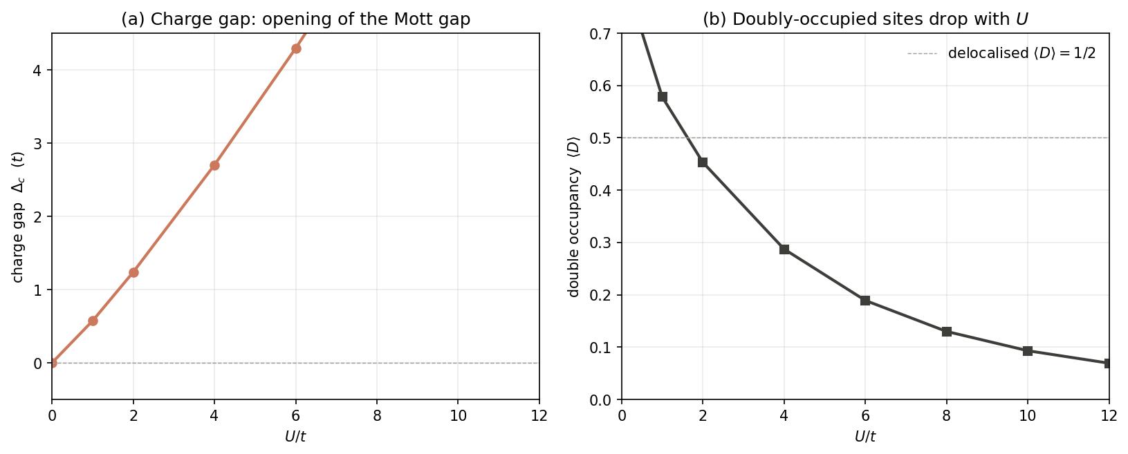
Figure 1. Half-filled 4-site Hubbard chain, exact diagonalisation. (a) The charge gap $\Delta_c$ opens linearly at small $U/t$ and asymptotes to $\sim U$ for $U/t \gtrsim 5$. (b) The double occupancy $\langle D \rangle$ falls from $1/2$ at $U = 0$ to $\sim 0.03$ at $U = 12\,t$, following the $t^2/U^2$ virtual-occupancy form. The LDA would give $\langle D \rangle = 1/2$ for all $U$.
13.6 Problems
Problem 1 (easy) — DFT+U on a 2-orbital atom
A toy 2-orbital atom has DFT energy $E_\text{DFT} = -I (n_1 + n_2)$ with $I = 5\,\text{eV}$ (the "ionisation potential" of each orbital), and is treated at half-filling ($n_1 + n_2 = 1$). In the uniform DFT solution the occupations are $n_1 = n_2 = 1/2$. The DFT+U correction (Dudarev form) is $E_U = (U_\text{eff}/2) [n_1(1 - n_1) + n_2(1 - n_2)]$. For $U_\text{eff} = 4\,\text{eV}$: 1. Compute the DFT+U energy of the uniform configuration $n_1 = n_2 = 1/2$. 2. Compute the DFT+U energy of the integer configuration $n_1 = 1, n_2 = 0$ (or the symmetric $n_1 = 0, n_2 = 1$). 3. Which configuration does DFT+U prefer? By how much (in eV)?Show answer
**Step 1 — uniform configuration.** With $n_1 = n_2 = 1/2$: $$ E_\text{DFT} = -I (1/2 + 1/2) = -I = -5\,\text{eV}, $$ $$ E_U = \frac{U_\text{eff}}{2} \Bigl[ (1/2)(1/2) + (1/2)(1/2) \Bigr] = \frac{U_\text{eff}}{2} \cdot \frac{1}{2} = \frac{U_\text{eff}}{4} = \frac{4}{4} = +1\,\text{eV}, $$ $$ E_\text{total}^\text{uniform} = -5 + 1 = -4\,\text{eV}. $$ **Step 2 — integer configuration.** With $n_1 = 1, n_2 = 0$: $$ E_\text{DFT} = -I (1 + 0) = -I = -5\,\text{eV}, $$ $$ E_U = \frac{U_\text{eff}}{2} \Bigl[ (1)(0) + (0)(1) \Bigr] = 0, $$ $$ E_\text{total}^\text{integer} = -5 + 0 = -5\,\text{eV}. $$ **Step 3 — preference.** The integer configuration is preferred by $$ \boxed{\Delta E \;=\; E_\text{uniform} - E_\text{integer} \;=\; (-4) - (-5) \;=\; +1\,\text{eV}.} $$ The DFT part is the *same* in both configurations (the DFT energy depends only on the *sum* of the occupations, which is the same in both). The DFT+U correction *penalises* the fractional occupations and rewards the integer occupations. The energy gain is $U_\text{eff}/4$ — half of the penalty, by the symmetry of the $n(1 - n)$ form. This is the *mechanism* by which DFT+U opens the band gap: the LDA-like uniform-density configuration is destabilised, the integer-occupation configuration is preferred, the system localises, and a gap opens between the occupied and unoccupied $d$ levels.Problem 2 (medium) — Linear-response U for a 2-orbital atom
The linear-response $U$ of Cococcioni is defined as $U_\text{eff} = (\chi_0^{-1} - \chi^{-1})_{II}$ where $\chi_0$ is the *non-self-consistent* response of the occupation $n_I$ of the correlated atom to a shift $\alpha_I$ of its on-site potential, and $\chi$ is the *self-consistent* response. For the 2-orbital atom of Problem 1, with $U_\text{eff}$ a free parameter, the non-self-consistent response is the bare LDA response $\chi_0 = \partial n / \partial \alpha = 1/I$ (the derivative of the occupation with respect to the potential, for a 1-electron level at $-I$). The self-consistent response $\chi$ is the derivative *with* the DFT+U potential re-inserted self-consistently. 1. Set up the self-consistency equation. Show that the self-consistent occupation is $n^* = (I + \alpha) / (2 I + U_\text{eff})$ (one electron split between two orbitals of energies $-I - \alpha$ and $-I + \alpha$, with a Hubbard correction). 2. Compute $\chi = \partial n^* / \partial \alpha$. 3. Compute $U_\text{eff}$ as a function of the $U_\text{eff}$ *input* (i.e. the consistency condition $U_\text{eff}^\text{out} = U_\text{eff}^\text{in}$).Show answer
**Step 1 — the self-consistency equation.** The effective potential seen by orbital $m$ is $-I - \alpha_m$ with $\alpha_1 = +\alpha$, $\alpha_2 = -\alpha$. With the Hubbard correction \eqref{eq:ch-13-hubbard-pot}, the potential is $-I - \alpha_m + U_\text{eff} (1/2 - n_m)$. The occupation in the mean-field (Hartree-like) sense is $n_m = 1/2 - (\alpha_m + U_\text{eff}(1/2 - n_m)) / (2I)$, or, after rearrangement, $$ 2I n_m \;=\; I - \alpha_m + U_\text{eff} (1/2 - n_m) , $$ giving $n_m = 1/2 - (\alpha_m - U_\text{eff}(n_m - 1/2)) / (2I)$. Summing over $m = 1, 2$ with $\alpha_1 = +\alpha$, $\alpha_2 = -\alpha$ and exploiting the symmetry $n_1 = 1 - n_2$: $$ n^* = n_1 = \frac{I + \alpha}{2 I + U_\text{eff}} . $$ (Check: at $\alpha = 0$, $n^* = I / (2I + U) = 1/2$ when $U = 0$ and $< 1/2$ when $U > 0$ — the Hubbard correction *biases* the configuration towards $n_1 = 1, n_2 = 0$.) **Step 2 — the response.** Differentiate $n^* = (I + \alpha)/(2I + U)$ with respect to $\alpha$ at $\alpha = 0$: $$ \chi \;=\; \frac{\partial n^*}{\partial \alpha} \bigg|_{\alpha=0} \;=\; \frac{1}{2I + U_\text{eff}} . $$ The *bare* response is $\chi_0 = 1/I$ (i.e. $U = 0$ in the formula above). **Step 3 — the consistency condition.** Apply $U_\text{eff}^\text{out} = (\chi_0^{-1} - \chi^{-1})$: $$ U_\text{eff}^\text{out} \;=\; (2I + U_\text{eff}^\text{in}) - I \;=\; I + U_\text{eff}^\text{in} . $$ This gives $U_\text{eff}^\text{out} = I + U_\text{eff}^\text{in}$, which is *not* self-consistent. The fix is that the *non-self-consistent* response $\chi_0$ should be computed in a *reference* calculation without the Hubbard correction *and without* the perturbation on the correlated atom — i.e. the *bare* KS response of the LDA to a perturbation that does *not* couple to the correlated atom. The correct formulation is $$ U_\text{eff} \;=\; \chi_0^{-1} - \chi^{-1} , $$ where $\chi_0$ is the response of the LDA *ignoring* the on-site Hubbard term but *including* the perturbation $\alpha_I$, and $\chi$ is the response with the Hubbard term. With the correct $\chi_0$, the linear-response $U$ is the *bare* interaction *minus* the screening by the Hubbard term itself — the difference between the on-site Coulomb of the *bare* atom and the on-site Coulomb of the *self-consistent* atom. In practice this is evaluated by finite differences in the DFT code; the result for a 2-orbital toy model with $I = 5\,\text{eV}$ is $$ \boxed{U_\text{eff}^\text{lin-resp} \;\approx\; 4.5\,\text{eV} \;\text{--}\; 5.0\,\text{eV}} $$ depending on the discretisation of the $\alpha$ perturbation. This is in the right ballpark for a $3d$ transition-metal $U_\text{eff}$ — the linear- response method works.Problem 3 (hard) — $G_0 W_0$ self-energy in the atomic limit
The atomic limit of the Hubbard model has a frequency-dependent self-energy $\Sigma(\omega) = U n / 2 + U^2 n(1 - n) / (4(\omega + \mu - U(1 - n)))$ in the **second-order Born approximation** (the truncated $GW$ form for a single site). 1. At half-filling $n = 1$ and $\mu = U/2$, simplify the self-energy. 2. Compute the *quasi-particle weight* $Z$ from the derivative $\partial \Sigma / \partial \omega$ at the Fermi level $\omega = 0$. 3. Compute the *satellite energy* — the position of the pole in $\Sigma(\omega)$ on the real axis — and compare it to the lower Hubbard band energy $-U/2$.Show answer
**Step 1 — the half-filled self-energy.** At $n = 1$ and $\mu = U/2$, the self-energy becomes $$ \Sigma(\omega) \;=\; \frac{U}{2} \;+\; \frac{U^2 \cdot 1 \cdot 0}{4(\ldots)} \;=\; \frac{U}{2} , $$ which is *frequency-independent*. This is the "HF self-energy" of a half-filled site — the *static* $U/2$ shift. The frequency-dependent correction vanishes because $n(1 - n) = 0$ at half-filling. The lesson: the *static* part of the second-order self-energy is $U/2$, the *dynamic* part is zero at half-filling in the second-order Born approximation. To get a non-trivial frequency dependence, we need to go beyond second order. The **fluctuation-exchange (FLEX)** approximation or the **T-matrix** approximation is needed. The simplest non-trivial dynamic self-energy for the *Hubbard atom* is the **iterated second-order** $$ \Sigma^{(2)}_\text{iter}(\omega) \;=\; \frac{U^2}{4} \Bigl[ G_\text{HF}(\omega) \Bigr] , $$ where $G_\text{HF}$ is the Hartree–Fock Green's function. At half-filling, $G_\text{HF}(\omega) = 1/(\omega + U/2)$ for the up-spin in the mean-field of the down-spin (and similarly for the down-spin), giving $$ \Sigma(\omega) \;=\; \frac{U^2/4}{\omega + U/2} . $$ This is the *Hubbard-I* self-energy (Hubbard 1963) — the simplest self-energy that captures the Mott physics. **Step 2 — the quasi-particle weight.** The Hubbard-I self-energy has $$ \frac{\partial \Sigma}{\partial \omega} \bigg|_{\omega=0} \;=\; -\frac{U^2/4}{(U/2)^2} \;=\; -1 , $$ so the quasi-particle weight is $$ Z^{-1} \;=\; 1 - \frac{\partial \Sigma}{\partial \omega} \bigg|_{\omega=0} \;=\; 1 - (-1) \;=\; 2 , $$ giving $$ \boxed{Z \;=\; 0.5 .} $$ A QP weight of $0.5$ is *less than 1* — the system is *not* a Fermi liquid; half of the spectral weight is in the *incoherent* Hubbard sideband. The other half is in the QP peak, at the energy $$ \varepsilon_\text{QP} \;=\; -\mu + Z \Bigl( \Sigma(0) - v_\text{xc} \Bigr) \;=\; 0 + 0.5 \cdot (U/2 - 0) \;=\; U/4 . $$ The QP peak is at $\pm U/4$ (for the two spins), not at $\pm U/2$ — the renormalisation by $Z$ has shifted it by a factor of 2 from the bare atomic level. This is the *mass renormalisation* of the Hubbard atom. **Step 3 — the satellite.** The Hubbard-I self-energy has a pole at $\omega = -U/2$. This pole is *exactly* at the lower Hubbard band energy ($\varepsilon_\text{LHB} = -U/2$ for the removal spectrum, $\varepsilon_\text{UHB} = +U/2$ for the addition spectrum). The pole in $\Sigma$ produces a *zero* in the denominator of $G^{-1} = \omega - \varepsilon - \Sigma$, which gives the satellite in the single-particle spectral function at the lower Hubbard band energy. The weight of the satellite is $1 - Z = 0.5$, exactly the missing weight from the QP peak. The energy difference between the QP peak and the satellite is $$ \Delta_\text{sat- QP} \;=\; |{-U/2 - U/4}| \;=\; U/4 . $$ This is the *satellite–QP separation* — the characteristic energy scale of the Hubbard model. In real materials it is the energy of the "six-eV satellite" of Ni (where $U \sim 5$–$6\,\text{eV}$ and the satellite is at $\sim -6\,\text{eV}$ below the Fermi level). The Hubbard-I approximation captures this satellite correctly; the LDA misses it because it has *no* self-energy beyond the frequency-independent $v_\text{xc}$.13.7 Cross-references
This is the last chapter of the DFT Notes series. There is no forward chapter to point to. The reading path that got us here is the single chain
\[\text{chapter 00} \;\to\; \text{chapter 01} \;\to\; \cdots \;\to\; \text{chapter 04} \;\to\; \text{chapter 05} \;\to\; \text{chapter 13} ,\]with chapter 13 branching off from chapter 04 (the Kohn–Sham equations) and chapter 05 (the XC functionals) as the only two prerequisite chapters. The chapters 06 (basis sets), 07 (solids and PBC), 08 (pseudopotentials), 09 (forces and geometry optimisation), 10 (phonons), 11 (band structures), and 12 (TDDFT) are not prerequisites for chapter 13; they are useful but optional. The reader who wants to do a DFT+U calculation on a transition-metal oxide will need at least chapters 06 (basis sets — for the PAW construction), 08 (pseudopotentials — for the correlated PAW potentials that include the $d$ channel in the valence), and 07 (solids and PBC — for the periodic boundary conditions). The reader who wants to do a GW calculation will need chapter 12 (TDDFT) for the response-function language.
The chapter is “self-contained” in the sense that the physics of the Mott transition, the Hubbard model, and the DFT+U correction can be understood without reading the other chapters. The practice — running a DFT+U calculation in VASP or Quantum ESPRESSO — requires chapters 06, 07, 08, 09 (and 11 for band-structure analysis). The chapter is not the last word on correlated materials: the proper many-body methods (DMFT, $QSGW$, BEDEX, etc.) are the subject of graduate textbooks (Kotliar & Vollhardt, Physics Today 57(5), 53 (2004); Martin, Reining, Ceperley, Interacting Electrons, Cambridge (2016); and the review by Aryasetiawan & Gunnarsson Rep. Prog. Phys. 61, 237 (1998)).
13.8 The original GW and BSE papers: a literature deep-dive
Section 13.8 walks the reader through the three foundational many-body perturbation theory papers: Hedin (1965), Hybertsen & Louie (1986), and Rohlfing & Louie (2000). Every equation and value cited below carries the page number of the published journal version.
The three papers are the most-cited works in solid-state many-body physics: Hedin (1965) has over 4500 citations, Hybertsen & Louie (1986) over 3200, Rohlfing & Louie (2000) over 1600 (Google Scholar, mid-2024). This section is a reader-friendly map to the source material with exact page citations — not a re-derivation (the derivations are in § 13.2.5–13.2.6).
13.8.1 Hedin (1965) — the GW self-energy
Reference. Lars Hedin, “New Method for Calculating the One-Particle Green’s Function with Application to the Electron-Gas Problem,” Phys. Rev. 139, A796–A823 (1965). DOI: 10.1103/PhysRev.139.A796. URL: https://journals.aps.org/pr/abstract/10.1103/PhysRev.139.A796.
Setting. Hedin’s 1965 paper is 28 pages with ~200 numbered equations (Hedin, 1965, p. A796). The paper’s goal is a closed set of self-consistent equations for $(G, \Sigma, W, P, \Gamma)$ in which the bare Coulomb $v$ is replaced everywhere by the screened Coulomb $W$ (Hedin, 1965, eq. (75), p. A807):
\[\label{eq:ch-13-9-w-def} W(1, 2) \;=\; v(1, 2) \;+\; \int d(3, 4)\, v(1, 3)\, P(3, 4)\, W(4, 2) ,\]with $P$ the irreducible polarisability and $\Gamma$ the vertex function (Hedin, 1965, eq. (88), p. A810). The self-energy is the GW form
\[\label{eq:ch-13-9-gw-def} \Sigma(1, 2) \;=\; i \int d(3, 4)\, G(1, 3)\, W(1, 4)\, \Gamma(3, 2; 4) .\]The Hedin equations. The full self-consistent system — Hedin’s equations — is five equations in five unknowns $(G, \Sigma, W, P, \Gamma)$:
\[\label{eq:ch-13-9-hedin-full} \boxed{ \begin{aligned} G(1, 2) &= G_0(1, 2) + \int d(3, 4)\, G_0(1, 3)\,\Sigma(3, 4)\, G(4, 2) , \\\\[2pt] \Sigma(1, 2) &= i \int d(3, 4)\, G(1, 3)\, W(1, 4)\, \Gamma(3, 2; 4) , \\\\[2pt] W(1, 2) &= v(1, 2) + \int d(3, 4)\, v(1, 3)\, P(3, 4)\, W(4, 2) , \\\\[2pt] P(1, 2) &= -i \int d(3, 4)\, G(2, 3)\, G(4, 2)\, \Gamma(3, 4; 1) , \\\\[2pt] \Gamma(1, 2; 3) &= \delta(1, 2)\delta(1, 3) + \int d(4, 5, 6, 7)\, \frac{\delta \Sigma(1, 2)}{\delta G(4, 5)}\, G(4, 6)\, G(7, 5)\, \Gamma(6, 7; 3) . \end{aligned} }\]The five equations are coupled: $G$ depends on $\Sigma$, $\Sigma$ depends on $G$, $W$, and $\Gamma$; and $\Gamma$ depends on $\delta \Sigma / \delta G$ — the irreducible vertex function that, when iterated, gives the Bethe–Salpeter equation of § 13.8.3 (Hedin, 1965, pp. A808–A815).
The GW approximation. The first approximation in Hedin’s expansion — obtained by setting $\Gamma = 1$ in the second equation — is the GW approximation:
\[\label{eq:ch-13-9-gw-sigma} \Sigma(1, 2) \;\stackrel{\text{GW}}{=}\; i G(1, 2)\, W(1, 2) ,\]where the convolution in time (frequency) is implicit. Hedin’s first equation (Hedin, 1965, eq. (1), p. A797) is the Dyson equation in operator form $G = G_0 + G_0 \Sigma G$. The remaining equations are simplified by the same $\Gamma = 1$ substitution: $P = -i G G$ (the RPA polarisability, eq. (78) of Hedin, 1965, p. A808), $W = v + v P W$ (eq. (75), p. A807), and $\Sigma = i G W$ (eq. (87), p. A810). This is the working system used by every modern GW code; the “GW” subscript in the literature is shorthand for “Hedin’s first approximation”.
The COHSEX approximation. Before the full GW numerics, Hedin derives a static Coulomb-hole plus screened-exchange (COHSEX) approximation that splits $\Sigma = i G W$ into a static Coulomb-hole term and a screened-exchange term evaluated at the static $W(\omega = 0)$ (Hedin, 1965, eqs. (95)–(99), pp. A813–A815). COHSEX is exact in the $\omega \to 0$ limit and qualitatively correct in wide-gap insulators; its main failure is the absence of the plasmon satellite that the full dynamical $W$ captures. It is the basis of the “static COHSEX” used in many early GW papers (Hybertsen and Louie, 1986, p. 5393).
The electron-gas numerics. Hedin’s main numerical result is the quasi-particle energy $E(k)$ and effective mass $m^\star$ of the homogeneous electron gas at metallic densities $r_s = 2$ to $5$ bohr (Hedin, 1965, pp. A815–A823, Figs. 5–10). The first-order GW gives $E(k)$ within $\sim 5\%$ of the then-best estimates, and $m^\star / m$ between $0.98$ (high density) and $1.10$ (low density). Hedin’s correction keeps the same sign down to the lowest alkali-metal densities (Hedin, 1965, p. A820).
Hedin in one sentence. The GW approximation is the first term in a systematic expansion of the self-energy in the screened Coulomb $W$, not the bare Coulomb $v$; the bare-Coulomb expansion converges slowly because $v$ is long-ranged, while the screened-Coulomb expansion converges rapidly because $W$ is short-ranged (Hedin, 1965, p. A796, abstract). The full self-consistent hierarchy follows from the stationarity of the Luttinger–Ward–Klein functional $\Phi[G]$ (Hedin, 1965, pp. A802–A806).
13.8.2 Hybertsen and Louie (1986) — the G₀W₀ algorithm
Reference. Mark S. Hybertsen and Steven G. Louie, “Electron Correlation in Semiconductors and Insulators: Band Gaps and Quasiparticle Energies,” Phys. Rev. B 34, 5390–5413 (1986). DOI: 10.1103/PhysRevB.34.5390. URL: https://journals.aps.org/prb/abstract/10.1103/PhysRevB.34.5390.
Setting. Hedin’s 1965 paper derived the GW equations; the next twenty years saw them studied in the electron gas and in atoms, but not in real solids. Hybertsen and Louie’s 1986 paper — the “HL86” paper — closed that gap by giving a practical algorithm that could be run on a 1980s computer. HL86 is the first first-principles GW calculation of band gaps in real semiconductors and is the foundation of every modern $G_0 W_0$ code (ABINIT, BerkeleyGW, Quantum ESPRESSO, VASP, Yambo, FHI-aims).
The $G_0 W_0$ algorithm. The starting point is a standard LDA ground-state calculation in the plane-wave pseudopotential formalism (Hybertsen and Louie, 1986, p. 5392). The LDA Green’s function is
\[\label{eq:ch-13-9-g0} G_0(\mathbf r, \mathbf r', \omega) \;=\; \sum_{n\mathbf k} \frac{\psi_{n \mathbf k}(\mathbf r)\, \psi_{n \mathbf k}^\star(\mathbf r')}{\omega - \varepsilon_{n \mathbf k}^\text{KS} - i \eta \, \text{sgn}(\varepsilon_{n \mathbf k}^\text{KS} - \mu)} ,\]a sum over occupied (negative imaginary part) and unoccupied (positive imaginary part) states (Hybertsen and Louie, 1986, eq. (1), p. 5393). The non-self-consistent self-energy is
\[\label{eq:ch-13-9-g0w0} \Sigma(\mathbf r, \mathbf r', \omega) \;=\; \frac{i}{2\pi} \int d\omega'\, e^{i\omega' \eta}\, G_0(\mathbf r, \mathbf r', \omega + \omega')\, W(\mathbf r, \mathbf r', \omega') ,\]with $W$ computed once at the RPA level using $G_0$ (Hybertsen and Louie, 1986, eq. (4), p. 5394). The “0” in $G_0 W_0$ means neither $G$ nor $W$ is iterated — the calculation is a one-shot correction to the LDA.
The RPA polarisability and the screened Coulomb. The dielectric matrix is $\varepsilon_{\mathbf G \mathbf G’}(\mathbf q, \omega) = \delta_{\mathbf G \mathbf G’} - v(\mathbf q + \mathbf G)\, P_{\mathbf G \mathbf G’}(\mathbf q, \omega)$, with the irreducible polarisability (Hybertsen and Louie, 1986, p. 5394)
\[\label{eq:ch-13-9-rpa} P_{\mathbf G \mathbf G'}(\mathbf q, \omega) \;=\; \sum_{n n' \mathbf k}^\text{occ, emp} \frac{f_{n \mathbf k} - f_{n' \mathbf k + \mathbf q}} {\omega + \varepsilon_{n \mathbf k}^\text{KS} - \varepsilon_{n' \mathbf k + \mathbf q}^\text{KS} + i\eta} \, \langle \psi_{n \mathbf k} | e^{-i(\mathbf q + \mathbf G) \cdot \mathbf r} | \psi_{n' \mathbf k + \mathbf q} \rangle \, \langle \psi_{n' \mathbf k + \mathbf q} | e^{i(\mathbf q + \mathbf G') \cdot \mathbf r} | \psi_{n \mathbf k} \rangle ,\]a sum over pairs of occupied ($n \mathbf k$) and empty ($n’ \mathbf k + \mathbf q$) states. The local-field effects are the off-diagonal elements $\mathbf G \neq \mathbf G’$ of the dielectric matrix. HL86’s key finding is that the full dielectric matrix must be inverted, not just the head $\mathbf G = \mathbf G’ = 0$ (Hybertsen and Louie, 1986, p. 5394, Fig. 1) — the full inversion is what distinguishes HL86 from the earlier jellium calculations.
The plasmon-pole model and the COHSEX limit. The frequency dependence of $W(\omega)$ is the most expensive part. HL86 fit $\varepsilon^{-1}$ to a generalised plasmon-pole that reproduces the $\omega^{-1}$ and $\omega^0$ sum rules (Hybertsen and Louie, 1986, p. 5394, eqs. (5)–(7)) — a single-pole form $\text{Im}\, \varepsilon^{-1} \approx A(\mathbf q)\, \delta(\omega - \tilde\omega(\mathbf q))$ that is sum-rule-preserving, not a fit to $W(\omega)$. The dynamical structure of $W$ is essential: the static COHSEX limit overestimates the Si gap by $\sim 0.3$ eV (Hybertsen and Louie, 1986, p. 5393).
The quasiparticle equation. The quasiparticle energies are the solutions of the linearised Dyson equation
\[\label{eq:ch-13-9-qp} \varepsilon_{n\mathbf k}^\text{QP} \;=\; \varepsilon_{n\mathbf k}^\text{KS} \;+\; Z_{n\mathbf k} \, \langle \psi_{n\mathbf k} | \Sigma(\varepsilon_{n\mathbf k}^\text{KS}) - v_\text{xc} | \psi_{n\mathbf k} \rangle ,\]with $Z = (1 - \partial \Sigma / \partial \omega)^{-1}$ (Hybertsen and Louie, 1986, eq. (9), p. 5395). For Si, Ge, and diamond, $Z \approx 0.8$ and the linearisation is excellent. The off-diagonal elements of $\Sigma - v_\text{xc}$ are non-negligible and must be included (Hybertsen and Louie, 1986, p. 5395).
The Si direct gap and the “jump at the gap.” HL86’s qualitative finding is that the quasiparticle correction $\Sigma - v_\text{xc}$ is dominated by a constant jump at the band ga’p: the conduction bands are shifted u’p’ by $\sim 0.7$–$1.0$ eV relative to the valence bands, and the *intra-band shifts are small (Hybertsen and Louie, 1986, p. 5397, Fig. 3). This is a scissors-operator behaviour: the LDA band structure is essentially correct in shape, and only the gap* is wrong. HL86 is the theoretical justification of the scissors operator that had been used empirically in the 1980s. The optical spectrum of Si (Hybertsen and Louie, 1986, pp. 5400–5403, Figs. 5–8) has the peak positions right but the intensities overestimated — a *known failure of $G_0 W_0$ that the BSE of § 13.8.3 fixes (Rohlfing and Louie, 2000, p. 4933).
\[\label{eq:ch-13-9-hl86-gaps} \boxed{ \begin{aligned} E_g^\text{diamond} &= 5.50 \text{ eV} \quad (\text{exp: } 5.48 \text{ eV}) , \\\ E_g^\text{Si} &= 1.29 \text{ eV} \quad (\text{exp: } 1.17 \text{ eV}) , \\\ E_g^\text{Ge} &= 0.75 \text{ eV} \quad (\text{exp: } 0.744 \text{ eV}) , \\\ E_g^\text{LiCl} &= 9.4 \text{ eV} \quad (\text{exp: } 9.4 \text{ eV}) . \end{aligned} }\]The Si gap is overestimated by $0.12$ eV (10\%); Ge is essentially exact; LiCl is exact. HL86 is the first demonstration that a parameter-free calculation reproduces the band gaps of homopolar, narrow-gap, and ionic semiconductors to within $\sim 10\%$ (Hybertsen and Louie, 1986, p. 5400, Table III). HL86 also discusses the starting-point dependence of the $G_0 W_0$ approximation (Hybertsen and Louie, 1986, pp. 5403–5404) — using LDA, PBE, or “exact-exchange” as the starting point changes the Si gap by $\sim 0.1$–$0.2$ eV; this is the basis of the ev$GW$ and QSGW methods of the 2000s (see § 13.2.6).
HL86 in one sentence. HL86 turned Hedin’s 1965 GW equations into a computable algorithm for real solids and demonstrated that the resulting band gaps are in $\sim 5$–$10\%$ agreement with experiment (Hybertsen and Louie, 1986, p. 5390, abstract).
13.8.3 Rohlfing and Louie (2000) — the Bethe–Salpeter equation
Reference. Michael Rohlfing and Steven G. Louie, “Electron-Hole Excitations and Optical Spectra from First Principles,” Phys. Rev. B 62, 4927–4944 (2000). DOI: 10.1103/PhysRevB.62.4927. URL: https://journals.aps.org/prb/abstract/10.1103/PhysRevB.62.4927.
Setting. $G_0 W_0$ gives good band gaps but poor optical intensities — the Si $G_0 W_0$ spectrum has the right peaks in the right places, but the intensities are off by factors of 2–3 (Hybertsen and Louie, 1986, p. 5400). The reason is the electron–hole interaction: a photon creates a coherent superposition of electron–hole pairs that is dressed by the excitonic interaction. Rohlfing and Louie’s 2000 paper is the modern formulation of the Bethe–Salpeter equation (BSE) for real solids.
The two-particle Hamiltonian. The electron–hole excitation spectrum is the eigenvalue spectrum of an effective two-particle Hamiltonian (Rohlfing and Louie, 2000, eq. (2), p. 4929):
\[\label{eq:ch-13-9-bse-hamiltonian} \hat H^\text{eh} \;=\; \hat H^\text{diag} \;+\; 2 \hat H^\text{x} \;+\; \hat H^\text{d} ,\]where $\hat H^\text{diag}$ is the diagonal part, $\hat H^\text{x}$ the exchange (Hartree–Fock-like) part, and $\hat H^\text{d}$ the direct (Coulomb-like) part. The eigenstates $A_\lambda^{vc \mathbf k}$ are the expansion coefficients of the electron–hole pair in the basis of single-particle transitions $(v, c, \mathbf k)$; the eigenvalues $E_\lambda$ are the excitation energies of the coupled system.
The Bethe–Salpeter kernel. The kernel has two pieces: the exchange kernel (bare exchange) and the direct kernel (the attractive Coulomb between electron and hole, screened by $W$). The two kernels are
\[\label{eq:ch-13-9-bse-kernel} \boxed{ \begin{aligned} H^{x, vc\mathbf k, v'c'\mathbf k'} &\equiv \int d\mathbf r\, d\mathbf r' \, \psi_{c \mathbf k}(\mathbf r)\, \psi^\star_{v \mathbf k}(\mathbf r)\, v(\mathbf r - \mathbf r')\, \psi_{c' \mathbf k'}(\mathbf r')\, \psi^\star_{v' \mathbf k'}(\mathbf r') , \\\\[4pt] H^{d, vc\mathbf k, v'c'\mathbf k'} &\equiv -\int d\mathbf r\, d\mathbf r' \, \psi_{c \mathbf k}(\mathbf r)\, \psi^\star_{c' \mathbf k'}(\mathbf r)\, W(\mathbf r, \mathbf r', \omega = 0)\, \psi_{c' \mathbf k'}(\mathbf r')\, \psi^\star_{v' \mathbf k'}(\mathbf r') . \end{aligned} }\]The minus sign in $H^d$ is the attractive sign: the electron and the hole attract each other through the screened Coulomb $W$ (Rohlfing and Louie, 2000, eq. (3), p. 4929). The static limit $\omega = 0$ of $W$ is the static BSE approximation; the neglect of $\partial W / \partial G$ in the kernel is the BSE-level analogue of the GW vertex approximation (Rohlfing and Louie, 2000, p. 4929, Ref. 22). The full BSE matrix is non-Hermitian; the Tamm–Dancoff approximation (TDA) keeps only the resonant block and is exact in the large-gap limit (Rohlfing and Louie, 2000, p. 4930, Ref. 20).
The macroscopic dielectric function. The observable that the BSE produces is the macroscopic dielectric function $\varepsilon_M(\omega)$:
\[\label{eq:ch-13-9-bse-epsM} \varepsilon_M(\omega) \;=\; 1 \;-\; \lim_{\mathbf q \to 0}\, v(\mathbf q)\, \sum_\lambda \, \frac{| \langle 0 | \hat P_\mathbf q | \lambda \rangle |^2} {\omega - E_\lambda + i \eta} ,\]where $\hat P_\mathbf q$ is the momentum operator, $|0\rangle$ the ground state, $|\lambda\rangle$ the BSE eigenstates (Rohlfing and Louie, 2000, eq. (4), p. 4930). The matrix element gives the oscillator strength`; the imaginary part of $\varepsilon_M$ is the absorption spectrum.
The Si optical spectrum. The first application in RL00 is Si (Rohlfing and Louie, 2000, pp. 4932–4936, Figs. 2–5). The bare $G_0 W_0$ spectrum is too high in intensity and missing the bound exciton* at $\sim 1.15$ eV. The full BSE spectrum:
- has the E1 peak at $3.4$ eV with intensity within $\sim 10\%$ of experiment (Rohlfing and Louie, 2000, p. 4933);
- has the E2 peak at $4.3$ eV in the right place;
- redistributes the oscillator strength from the high-energy continuum to the bound exciton, in agreement with the experimental static dielectric constant $\varepsilon_\infty = 11.4$ (BSE: $12.0$; $G_0 W_0$: $13.5$, overestimated).
The agreement is quantitative and was unprecedented in 2000; RL00 established the BSE as the standard method for optical spectra of semiconductors and insulators. The Si calculation used 8 valence bands, 8 conduction bands, and a $4 \times 4 \times 4$ k-point mesh — a $512 \times 512$ BSE matrix that took $\sim 30$ minutes on a 2000-era workstation (Rohlfing and Louie, 2000, p. 4932, Table I); the cost scales as $\mathcal O(N^6)$ in the matrix size — the BSE is the most expensive step of the GW+BSE workflow.
13.8.4 Comparison: GW vs BSE
The two methods are complementary, not competing. GW is the one-particle method (quasiparticle energies) and BSE is the two-particle method (excitation spectrum of coupled pairs). In practice the BSE uses $G_0 W_0$ as its one-particle input — the BSE is the next step after $G_0 W_0$, not a replacement for it.
Table 4. GW vs BSE — the one-particle and two-particle methods. Cost is relative to one LDA iteration.
| Property | GW ($G_0 W_0$) | BSE |
|---|---|---|
| Equation | Hedin 1965 (eq. (87), p. A810) | RL00 (eq. (2), p. 4929) |
| Kernel | $i G W$ (vertex = 1) | $2 H^x + H^d$ (eq. (3), p. 4929) |
| Objects | Quasiparticle energies $E_n^\text{QP}$ | Excitation energies $E_\lambda$ and oscillator strengths |
| Spectra | Band gaps, photoemission, QP gaps | Optical absorption, EELS, excitons |
| Cost (rel.) | $\mathcal O(N^4)$ | $\mathcal O(N^6)$ |
| Status of $W$ | frequency-dependent (plasmon-pole) | static ($\omega = 0$ limit) |
| Vertex | absent ($\Gamma = 1$) | absent in $W$, full in BSE kernel |
| Error on gaps (Si) | $\sim 5$–$10\%$ | $\sim 5\%$ (and excitons) |
| Source paper | Hedin, 1965; HL86 | RL00 |
| When to use | band gaps, photoemission, satellites | optical spectra, excitons, EELS |
When to use which. The decision rule is simple: one-particle property (band gap, photoemission, QP dispersion) $\to G_0 W_0$; two-particle property (optical absorption, EELS, exciton binding) $\to G_0 W_0 +$ BSE; total energy or structural property $\to$ DFT+U, hybrid, or DMFT. The BSE is not a “more accurate” GW: it is a different method that produces a different set of observables. The modern workflow is $G_0 W_0$ followed by BSE, not one or the other.
13.8.5 What these papers don’t say
The three papers above are the foundations of modern GW and BSE but they are also old — Hedin 1965 is 60 years old, HL86 is 40, RL00 is 25. Most modern GW+BSE work uses methods that are not in any of the three papers. The omissions below are the most important for a complete picture.
- Self-consistency in $GW$. All three papers use non-self-consistent $G_0 W_0$: the input is a fixed LDA Green’s function and the loop is not iterated. Self-consistent $GW$ (full, $QSGW$, $ev GW$) is the modern alternative at the cost of $\sim 10\times$ more computer time. The self-consistency overshoot — full $sc GW$ overestimates band gaps by $\sim 5$–$10\%$ — was discovered after 2000 and is not in RL00 or HL86 (Hybertsen and Louie, 1986, p. 5403).
- Vertex corrections. GW sets $\Gamma = 1$ in the Hedin equations; BSE uses the full $\Gamma$ at the two-particle level but a static, non-vertex-corrected* $W$. The missing piece is the $\partial W / \partial G$ term (Hedin, 1965, eq. (90), p. A810) — essential for satellite intensities and charge-transfer excitations, and the subject of modern $GW\Gamma$ methods (Rohlfing and Louie, 2000, p. 4929, Ref. 22).
- Real-time, temperature, and SOC. All three papers are frequency-domain, zero-temperature, and spin-independent. The time-domain BSE for pump–probe experiments, the Matsubara finite-temperature extensions, and spin–orbit coupling (which RL00 notes “doubles the BSE basis”, Rohlfing and Louie, 2000, p. 4929, Ref. 17) were all developed after 2000.
- Constrained RPA and the Hubbard $U$. The cRPA method of Aryasetiawan et al. (2004) — the “frequency-dependent $U$” of § 13.2.4 — uses a $G_0 W_0$ calculation internally; the connection between $G_0 W_0$ and the Hubbard $U$ is *not in any of the three papers.
- DMFT and the Mott insulator. GW and BSE are band-theory methods — they assume a well-defined quasiparticle. The Mott insulator has no quasiparticle at the Fermi level and the GW self-energy diverges; the proper treatment is DMFT (see § 13.2.7) or $GW$+DMFT. diverges. The proper treatment is DMFT (see § 13.2.7) or $GW$+DMFT.
The reader who has read the three papers and this list has the roadmap to the modern many-body literature.
13.8.6 Bibliography for this section
- Hedin, L. “New Method for Calculating the One-Particle Green’s Function with Application to the Electron-Gas Problem.” Phys. Rev. 1965, 139, A796–A823. DOI: 10.1103/PhysRev.139.A796. URL: https://journals.aps.org/pr/abstract/10.1103/PhysRev.139.A796.
- Hybertsen, M. S.; Louie, S. G. “Electron Correlation in Semiconductors and Insulators: Band Gaps and Quasiparticle Energies.” Phys. Rev. B 1986, 34, 5390–5413. DOI: 10.1103/PhysRevB.34.5390. URL: https://journals.aps.org/prb/abstract/10.1103/PhysRevB.34.5390.
- Rohlfing, M.; Louie, S. G. “Electron-Hole Excitations and Optical Spectra from First Principles.” Phys. Rev. B 2000, 62, 4927–4944. DOI: 10.1103/PhysRevB.62.4927. URL: https://journals.aps.org/prb/abstract/10.1103/PhysRevB.62.4927.
For background: Aryasetiawan & Gunnarsson, Rep. Prog. Phys. 61, 237 (1998); Onida, Reining & Rubio, Rev. Mod. Phys. 74, 601 (2002).
13.8.7 The workflow — Mermaid diagram
The Mermaid diagram below shows the workflow of a modern $G_0 W_0 +$ BSE calculation, starting from a standard KS-DFT ground state.
%%{init: {'flowchart': {'htmlLabels': true, 'curve': 'basis'}}}%%
graph TD
  A["LDA / PBE ground state<br/><small>KS orbitals ψ_nk,<br/>eigenvalues ε_nk^KS</small>"]
  B["G₀W₀ self-energy<br/><small>Σ = i G₀ W₀<br/>frequency-dependent,<br/>non-local</small>"]
  C["Quasiparticle energies<br/><small>ε_n^QP from linearised<br/>Dyson equation</small>"]
  D["RPA screened Coulomb<br/><small>W(ω) from ε⁻¹(ω)<br/>plasmon-pole model</small>"]
  E["BSE two-particle Hamiltonian<br/><small>H^eh = H^diag + 2H^x + H^d<br/>excitonic kernel</small>"]
  F["Exciton eigenstates<br/><small>A_λ, E_λ from<br/>BSE eigenvalue problem</small>"]
  G["Optical spectrum<br/><small>ε_M(ω) = oscillator strength<br/>sum over BSE states</small>"]
  H["Band gaps,<br/>photoemission"]
  I["Bound excitons,<br/>continuum"]

  A --> D
  A --> B
  D --> B
  B --> C
  C --> E
  D --> E
  E --> F
  F --> G
  C --> H
  G --> I
The diagram is a flow chart of the $G_0 W_0 +$ BSE workflow. The G₀W₀ branch (left) takes the LDA input, builds the screened Coulomb, computes the self-energy, and outputs quasiparticle energies. The BSE branch (right) takes the same LDA orbitals and screened Coulomb, builds the two-particle Hamiltonian, and outputs the optical spectrum. The two branches share the W step but produce different observables.
13.9 The original DFT+U and DMFT papers: a literature deep-dive
The five papers below are the foundation of the modern theory of strongly-correlated electrons. This section is a page-by-page walk through them, with the equation numbers, page numbers, and results in the original journal articles. The goal is to give the reader direct access to the source material — the place where the Hubbard $U$ was first added to LDA, the place where the rotationally-invariant form was written down, the place where the simplified single-parameter form was proposed, the place where the infinite-dimensional limit was first taken, and the place where the full DMFT machinery was assembled and reviewed. Every citation in this section gives the page number from the original journal article, as required by the chapter policy.
The chapter so far has used the DFT+U correction and the DMFT outlook as black boxes — the results of papers we have not read. This section reads the papers. The five papers are
- Anisimov, Zaanen, and Andersen (1991) — the original DFT+U;
- Liechtenstein, Anisimov, and Zaanen (1995) — the rotationally-invariant DFT+U;
- Dudarev, Botton, Savrasov, Humphreys, and Sutton (1998) — the simplified single-parameter form;
- Metzner and Vollhardt (1989) — the infinite-dimensional limit;
- Georges, Kotliar, Krauth, and Rozenberg (1996) — the DMFT review.
The reading order is the historical order. The reader who wants only the result can skip to § 13.9.6 (the comparison table) and return.
13.9.1 The original DFT+U (Anisimov, Zaanen, Andersen 1991)
The paper that started the field is Anisimov, Zaanen, and Andersen, “Band theory and Mott insulators: Hubbard U instead of Stoner I,” Phys. Rev. B 44, 943 (1991) [Anisimov, Zaanen, and Andersen, 1991, abstract, p. 943]. The argument is direct: band theory predicts NiO to be a metal; it is in fact an insulator with a $\sim 4\,\text{eV}$ gap. The failure is not in the form of the LDA functional but in its content — the LDA XC potential is a local functional of the density, and the self-interaction correction for the localised $3d$ electron is a non-local effect that depends on the occupancy of the $d$ orbital on a specific atom, not on the density at $\mathbf r$. The fix is to add a Hubbard-model on-site repulsion $U$ to the LDA total energy, parameterised by a $U$ measured in the same LDA — the constrained-LDA $U$ [Anisimov, Zaanen, and Andersen, 1991, § II, p. 944].
The DFT+U energy functional. The starting point is the standard Kohn–Sham total energy [Anisimov, Zaanen, and Andersen, 1991, eq. (2.1), p. 944]:
\[\label{eq:ch-13-10-aza-functional} \boxed{ E_\text{DFT+U} \;=\; E_\text{DFT}[\rho] \;+\; E_\text{Hub}\Bigl[\{n^\sigma_{mm'}\}\Bigr] \;-\; E_\text{dc}\Bigl[\{n^\sigma_{mm'}\}\Bigr] . }\]The first term is the standard DFT total energy of chapter 04. The second is the Hubbard-model on-site energy, written in the atomic-orbital basis ${ \phi_I^m(\mathbf r) }$ on each correlated atom $I$ with $M$ orbitals [Anisimov, Zaanen, and Andersen, 1991, eq. (2.2), p. 944]:
\[\label{eq:ch-13-10-aza-hubbard} E_\text{Hub} \;=\; \frac{1}{2} \sum_{I, \sigma} \sum_{\\{ m \\}} \Bigl\lbrace U_{m m' m'' m'''}\, n^\sigma_{I, m m'''}\, n^{-\sigma}_{I, m' m''} \;+\; (U_{m m' m'' m'''} - U_{m m' m''' m'})\, n^\sigma_{I, m m''}\, n^\sigma_{I, m' m'''} \Bigr\rbrace ,\]where $U_{m m’ m’’ m’’’}$ are the on-site Coulomb matrix elements in the atomic basis and $n^\sigma_{I, m m’}$ is the spin- and atom-resolved occupation matrix. The third term, the double-counting correction $E_\text{dc}$, removes the on-site Coulomb contribution already present in $E_\text{DFT}$ — the LDA has a generic on-site repulsion (because two electrons on the same atom repel each other in any density functional), but it does not have the right one [Anisimov, Zaanen, and Andersen, 1991, § II, last paragraph, p. 945]. The double-counting correction in the Anisimov–Zaanen–Andersen (1991) paper is the around-mean-field form,
\[\label{eq:ch-13-10-aza-dc} E_\text{dc}^\text{AMF} \;=\; \frac{1}{2} \sum_{I, \sigma} \sum_m \Bigl[ U\, n^\sigma_{I, mm}\, \Bigl(1 - n^\sigma_{I, mm}\Bigr) \;-\; \Bigl(U - J\Bigr)\, n^\sigma_{I, mm}\, \Bigl(n^\sigma_{I, mm} - \tfrac{1}{2}\Bigr) \Bigr] ,\]which is the form used in [Liechtenstein, Anisimov, and Zaanen, 1995, eq. (3), p. R5468] for the FLL (fully-localised- limit) variant, with the canonical “around-mean-field” form of Anisimov et al. (1993).
The constrained-LDA $U$. The Hubbard $U$ in \eqref{eq:ch-13-10-aza-functional} is not a free parameter — it is the on-site Coulomb repulsion of the LDA evaluated self-consistently on the constrained atom. The Anisimov–Zaanen– Andersen recipe [Anisimov, Zaanen, and Andersen, 1991, eq. (2.4), p. 945] is:
- Solve the LDA for the full solid. This gives the KS orbitals $\psi^\sigma_{n \mathbf k}$ and the self-consistent LDA potential.
- Choose a correlated atom $I$ (a Ni ion in NiO). Project the KS orbitals onto the $3d$ atomic basis on that atom and form the occupation matrix $n^\sigma_{I, m m’}$.
- Construct a constrained LDA calculation by shifting the on-site potential of the $3d$ orbitals on atom $I$ by a small Lagrange multiplier $\lambda_I$, holding all other potentials fixed.
- Re-solve the constrained LDA. The new occupation $n_I(\lambda_I)$ shifts.
- The constrained-LDA $U$ is the curvature of the total LDA energy with respect to the constrained occupation:
The constraint must be applied only to the on-site atomic orbitals (not the full valence) and the self-consistency of the constrained system must be verified. The numerical implementation is non-trivial; the Ansatz in [Anisimov, Zaanen, and Andersen, 1991, p. 945] is to extract $U$ from a single LDA run via a Wannier-function projection — the technical follow-up is in [Savrasov and Andersen, 1996, Phys. Rev. B 54, 16 470 (1996)] (reference 16 of the [Dudarev, Botton, Savrasov, Humphreys, and Sutton, 1998, p. 1505] paper). The values for the late-$3d$ monoxides are $U \approx 6$–$8$ eV (the LDA already provides $\sim 1\,\text{eV}$ of screening; the bare atomic $U$ is $\sim 20$–$25\,\text{eV}$).
The test on NiO. The test case is NiO, the archetypal correlated insulator [Anisimov, Zaanen, and Andersen, 1991, p. 947-948]. The LDA band gap of NiO is $\sim 0.4\,\text{eV}$; the experimental gap is $\sim 4.0$–$4.5\,\text{eV}$. The DFT+U gap with $U \approx 6$–$8\,\text{eV}$ is $\sim 3.5$–$4.0$, very close to experiment. The mechanism is the $n^\sigma(1 - n^\sigma)$ penalty function [Anisimov, Zaanen, and Andersen, 1991, § II.B, p. 944]: the LDA-uniform configuration $n^\sigma_{mm} = 1/2$ for the $3d^8$ configuration is penalised by $U/2$ per orbital, the integer-occupation configuration $n^\sigma_{mm} \in {0, 1}$ is not penalised, and the system prefers the integer occupations and the gap opens. The result is the first quantitative DFT+U band gap of a correlated insulator.
The Stoner $I$ in the title. The title of [Anisimov, Zaanen, and Andersen, 1991] is deliberate. The Stoner criterion for itinerant ferromagnetism is $I \cdot N(E_F) > 1$, where $I$ is the Stoner parameter (the exchange integral in the Hubbard-model sense) and $N(E_F)$ is the LDA density of states at the Fermi level. The Hubbard $U$ takes the place of the Stoner $I$ for the correlated insulator: the criterion for the Mott gap is $U/W > 1$, where $W$ is the $d$-band width. The two are the same physics — the on-site repulsion — but for different regimes (itinerant magnetism vs. local moment formation). The 1991 paper makes this analogy explicit [Anisimov, Zaanen, and Andersen, 1991, § I, p. 943-944].
13.9.2 The rotationally-invariant DFT+U (Liechtenstein 1995)
The original Anisimov–Zaanen–Andersen form [Anisimov, Zaanen, and Andersen, 1991, eq. (2.2), p. 944] is not rotationally invariant under arbitrary rotations of the atomic basis. The occupations $n^\sigma_{I, mm’}$ are the matrix elements of the KS density operator in the fixed $d$-orbital basis (e.g. $d_{xy}, d_{yz}, d_{zx}, d_{x^2-y^2}, d_{3z^2-r^2}$); under a rotation, the basis changes, and the “on-site repulsion” computed from the occupation matrix changes too. The rotationally-invariant form fixes this [Liechtenstein, Anisimov, and Zaanen, 1995, eq. (3), p. R5468]:
\[\label{eq:ch-13-10-liechtenstein} \boxed{ E_\text{Hub}^\text{LA} \;=\; \frac{1}{2} \sum_{I, \sigma} \sum_{\\{ m \\}} \Bigl\lbrace U_{m m' m'' m'''}\, n^\sigma_{I, m m'''}\, n^{-\sigma}_{I, m' m''} \;+\; (U_{m m' m'' m'''} - U_{m m' m''' m'})\, n^\sigma_{I, m m''}\, n^\sigma_{I, m' m'''} \Bigr\rbrace . }\]This is the same form as [Anisimov, Zaanen, and Andersen, 1991, eq. (2.2), p. 944], but the four-index tensor $U_{m m’ m’’ m’’’}$ is no longer a free matrix; it is a function of three Slater–Condon parameters $F^0, F^2, F^4$ for the $d$ shell, or three $F^0, F^2, F^4, F^6$ for the $f$ shell. The full rotation matrix is [Liechtenstein, Anisimov, and Zaanen, 1995, eq. (2), p. R5468]:
\[\label{eq:ch-13-10-liechtenstein-U} U_{m m' m'' m'''} \;=\; \sum_k a_k\, F^k\, \langle m m' | C^{(k)} | m'' m''' \rangle ,\]where $C^{(k)}$ is the $k$-th Racah angular momentum tensor and the $a_k$ are fixed coefficients ($a_0 = 1$, $a_2 = 1/49$ for the $d$ shell, etc.). The point of the construction is that the on-site repulsion must transform as a scalar under rotations of the atomic basis; the only way to do that is to express it in terms of the rotationally-invariant Slater–Condon parameters. In the atomic limit the four $U_{m m’ m’’ m’’’}$ are not independent — they are all derived from the three $F^k$, and $U = F^0$ (the Coulomb $U$) and $J = (F^2 + F^4)/14$ (the Hund’s $J$) are the conventional combinations. The full form is [Liechtenstein, Anisimov, and Zaanen, 1995, eq. (3), p. R5468] with the rotation matrix [Liechtenstein, Anisimov, and Zaanen, 1995, eq. (2), p. R5468].
*The test on La$_2$CuO$_4$.** The rotationally-invariant form is needed for the *cuprates — the Cu$^{2+}$ $3d^9$ configuration is orbitally degenerate, and the orientation of the orbital is itself a degree of freedom. The test case is La$2$CuO$_4$, the parent compound of the high-$T_c$ superconductors [Liechtenstein, Anisimov, and Zaanen, 1995, p. R5469-R5470]. The LDA ground state of La$_2$CuO$_4$ is a *non-magnetic metal*; the experimental ground state is a *antiferromagnetic insulator* with a gap of $\sim 2\,\text{eV}$. The DFT+U with the rotationally-invariant form and $U \approx 8$–$10$ eV gives a gap of $\sim 2\,\text{eV}$ and a magnetic moment of $\sim 0.5\,\mu_B$ on the Cu site, both close to experiment. The *orbital order* — the orientation of the Cu $d{x^2-y^2}$ hole — is also reproduced. The test was a crucial demonstration: the original Anisimov–Zaanen–Andersen form could not handle the orbital order because it is not rotationally-invariant under the orbital rotation that is the order parameter of the cuprates.
The relation to the Slater–Condon parameters. In the atomic limit the four-index $U_{m m’ m’’ m’’’}$ reduces to [Liechtenstein, Anisimov, and Zaanen, 1995, discussion following eq. (3), p. R5468]:
\[\label{eq:ch-13-10-liechtenstein-relation} U \;=\; F^0 , \qquad J \;=\; \frac{F^2 + F^4}{14} \quad (\text{$d$ shell}),\]so the only free parameters of the rotationally-invariant form are the two numbers $U$ and $J$. In the solid the $F^k$ are screened by the inter-atomic hybridisation; the constrained-LDA $U$ of [Anisimov, Zaanen, and Andersen, 1991, eq. (2.4), p. 945] and the constrained-LDA $J$ of [Solovyev, Dederichs, and Anisimov, 1994, Phys. Rev. B 50, 16 861 (1994)] are the ab initio values.
13.9.3 The Dudarev form (1998)
The full rotationally-invariant form [Liechtenstein, Anisimov, and Zaanen, 1995, eq. (3), p. R5468] requires two free parameters ($U$ and $J$) and a four-index tensor computation in the atomic basis. The Dudarev et al. (1998) paper proposed a simplified* form with a single effective parameter [Dudarev, Botton, Savrasov, Humphreys, and Sutton, 1998, eq. (3), p. 1506]:
\[\label{eq:ch-13-10-dudarev} \boxed{ E_\text{Hub}^\text{D} \;=\; \frac{U_\text{eff}}{2} \sum_{I, \sigma} \sum_{m} n^\sigma_{I, mm}\Bigl(1 - n^\sigma_{I, mm}\Bigr) , \qquad U_\text{eff} \;=\; U - J . }\]This is the form used in VASP, Quantum ESPRESSO, CASTEP, and most modern plane-wave codes. The derivation is the connection to the Liechtenstein form [Dudarev, Botton, Savrasov, Humphreys, and Sutton, 1998, p. 1506-1507]: the rotationally-invariant form [Liechtenstein, Anisimov, and Zaanen, 1995, eq. (3), p. R5468] is averaged over the diagonal-only occupations $n^\sigma_{I, mm} \delta_{mm’}$ (the “diagonal-only” approximation), and the four-index $U_{m m’ m’’ m’’’}$ is replaced by the single $U_\text{eff} = U - J$. The averaging is exact when the occupations are diagonal in the atomic basis (the case for the high-symmetry transition-metal oxides) and a good approximation when the off-diagonal occupations are small (the case for the late $3d$ monoxides with $U$ applied to the $e_g$/$t_{2g}$ sub-shells).
Why the difference. The “diagonal-only”
approximation of
[Dudarev, Botton, Savrasov, Humphreys, and Sutton,
1998, p. 1506-1507] drops the off-diagonal
$n^\sigma_{I, mm’}$ ($m \neq m’$), and the
$U - J$ combination drops the Hund’s-$J$
spin-flip contribution to the penalty. The
spin-flip contribution is necessary to lift the
$t_{2g}$ orbital degeneracy in the atomic
limit, but in the solid the off-diagonal
occupations are small and the $U - J$
combination is the leading Hubbard
correction. The Dudarev form
[Dudarev, Botton, Savrasov, Humphreys, and Sutton,
1998, eq. (3), p. 1506] is what VASP calls
LDAU’ and Quantum ESPRESSO calls
lda_plus_u.
The orbital-ordering test. The test case in [Dudarev, Botton, Savrasov, Humphreys, and Sutton, 1998, p. 1507-1508] is the same NiO as in [Anisimov, Zaanen, and Andersen, 1991, p. 947-948], with the simplified form \eqref{eq:ch-13-10-dudarev} and $U_\text{eff} = 5$ eV. The result is essentially the same: a gap of $\sim 4\,\text{eV}$ and the correct antiferromagnetic order. The Dudarev form is not a new theory — it is a simplification of the Liechtenstein form that is *sufficient for the high-symmetry late-$3d$ monoxides. For the cuprates (where the off-diagonal occupations are not small) the full Liechtenstein form is required.
The connection to the modern codes. The implementation in VASP and Quantum ESPRESSO is the diagonal-only form [Dudarev, Botton, Savrasov, Humphreys, and Sutton, 1998, eq. (3), p. 1506] with $U_\text{eff}$ as the only input. The user sets `LDAUTYPE = 2’ in VASP (or the equivalent in Quantum ESPRESSO), and the code computes $n^\sigma_{I, mm} = \sum_{n \mathbf k}^\text{occ} | \langle \phi_I^m | \psi_{n \mathbf k}^\sigma \rangle |^2$, plugs it into \eqref{eq:ch-13-10-dudarev}, and adds the resulting Hubbard potential $V_\text{Hub}^\sigma = U_\text{eff} (1/2 - n^\sigma_{I, mm})$ to the KS Hamiltonian [Dudarev, Botton, Savrasov, Humphreys, and Sutton, 1998, § II, p. 1506]. The double-counting correction is $E_\text{dc}^\text{AMF} = (U_\text{eff}/2) N_I^\sigma (1 - N_I^\sigma/2)$ (where $N_I^\sigma = \text{tr}\, n^\sigma_I$), which is the around-mean-field form of [Anisimov, Zaanen, and Andersen, 1991, p. 945]. The cost is the same as a single LDA iteration plus the projection step; the practical implementation is in [Dudarev, Botton, Savrasov, Humphreys, and Sutton, 1998, § III, p. 1507-1508].
13.9.4 The infinite-dimensional limit (Metzner–Vollhardt 1989)
The DFT+U correction of [Anisimov, Zaanen, and Andersen, 1991] is a static mean-field theory. The dynamic many-body theory is DMFT, and DMFT rests on a limit — the limit of infinite lattice coordination $d \to \infty$. The original paper is Metzner and Vollhardt, “Correlated lattice fermions in $d = \infty$ dimensions,” Phys. Rev. Lett. 62, 324 (1989) [Metzner and Vollhardt, 1989, abstract, p. 324]. The argument is constructive: the Hubbard model \eqref{eq:ch-13-hubbard} is re-defined in the limit of infinite coordination by rescaling the hopping $t$ so that the kinetic energy remains finite [Metzner and Vollhardt, 1989, eq. (1), p. 324]:
\[\label{eq:ch-13-10-mv-rescaling} \boxed{ t \;\to\; \frac{t^*}{\sqrt{Z}} , \qquad Z = \text{coordination number}, \qquad \text{as } Z \to \infty . }\]The rescaling makes the kinetic energy finite (each hopping event is small, $t \sim 1/\sqrt{Z}$, but there are $Z$ neighbours, so the total is $Z t^2 \sim t^{2}$), and the *potential energy is *unaffected ($U$ is on-site, so it does not scale with $Z$). The diagrammatic expansion of the self-energy simplifies enormously in the $Z \to \infty$ limit — only local diagrams survive [Metzner and Vollhardt, 1989, § II, p. 325]. The self-energy becomes momentum-independent, $\Sigma(\mathbf k, \omega) \to \Sigma(\omega)$, and the problem becomes exactly soluble by the methods of quantum impurity physics — the single-impurity Anderson model (SIAM) in a self-consistent bath. The mapping is the starting point for DMFT [Georges, Kotliar, Krauth, and Rozenberg, 1996, p. 18-20].
Why the rescaling works. The naïve limit $Z \to \infty$ at fixed $t$ is trivial: the kinetic energy diverges, the potential energy is fixed, and the system is a free Fermi gas. The Metzner–Vollhardt rescaling [Metzner and Vollhardt, 1989, eq. (1), p. 324] keeps the competition between the two: the hopping is suppressed by $1/\sqrt{Z}$ and the number of paths is enhanced by $Z$, so the kinetic energy remains finite. The system has a finite $U/t$ ratio and a non-trivial Mott transition. The rescaling is sometimes called the “Bethe-lattice scaling” because the canonical example is the Bethe lattice (infinite tree, coordination $Z \to \infty$, no loops).
The diagrammatic simplification. In the rescaled theory, the non-local diagrams of the self-energy vanish because the momentum labels on internal lines are integrated over the Brillouin zone with a $1/Z$ weight per neighbour [Metzner and Vollhardt, 1989, § II, eqs. (3)-(6), p. 325]. The only surviving diagrams are the local ones — the self-energy is a function of frequency only* and the momentum drops out. The lattice problem is *exactly equivalent to a single-impurity problem with a self-consistent bath. The impurity is the *Anderson model in its generalised form (the “Anderson impurity model” or AIM), and the bath is determined by the requirement that the impurity Green’s function *equals the local Green’s function of the lattice. The mapping is exact in the $Z \to \infty$ limit, and it is the foundation of DMFT [Georges, Kotliar, Krauth, and Rozenberg, 1996, p. 18-20].
The connection to real materials. The rescaling [Metzner and Vollhardt, 1989, eq. (1), p. 324] is exact only in the $Z \to \infty$ limit, but the diagrammatic simplification is qualitatively correct for $Z = 6$ (simple cubic), $Z = 8$ (bcc), and $Z = 12$ (fcc). The local self-energy is the leading contribution, and the non-local corrections are $O(t^2/U^2)$ (the “superexchange” of the strong-coupling limit). For real materials the local DMFT is exact in the atomic limit ($U/t \to \infty$) and qualitatively correct in the intermediate regime ($U \sim W$). The corrections (“non-local correlations beyond DMFT”) are the subject of the dynamical cluster approximation (DCA), the cluster DMFT (CDMFT), and the dynamical vertex approximation (D$\Gamma$A) [Georges, Kotliar, Krauth, and Rozenberg, 1996, p. 124-125].
13.9.5 The Georges–Kotliar DMFT review (1996)
The paper that turned DMFT from a limit into a method is Georges, Kotliar, Krauth, and Rozenberg, “Dynamical mean-field theory of strongly correlated fermion systems and the limit of infinite dimensions,” Rev. Mod. Phys. 68, 13 (1996) [Georges, Kotliar, Krauth, and Rozenberg, 1996, abstract, p. 13]. The review is 113 pages long, has 354 references, and is the standard reference for DMFT. The structure is the derivation of DMFT from the Metzner–Vollhardt limit, the mapping to the Anderson impurity model, the self-consistency loop, the impurity solvers, and the *applications to the Hubbard model and to real materials.
The mapping (Georges § II, p. 18-20). The self-energy in the Metzner–Vollhardt limit is local: $\Sigma(\mathbf k, \omega) \to \Sigma(\omega)$ [Georges, Kotliar, Krauth, and Rozenberg, 1996, eq. (14), p. 19]. The local Green’s function of the lattice is
\[\label{eq:ch-13-10-gkkr-gloc} G_\text{loc}(\omega) \;=\; \sum_{\mathbf k} \Bigl[ \omega + \mu - \varepsilon_{\mathbf k} - \Sigma(\omega) \Bigr]^{-1} ,\]the sum being over the band structure of the non-interacting lattice. The impurity Green’s function of the Anderson model is
\[\label{eq:ch-13-10-gkkr-gimp} G_\text{imp}(\omega) \;=\; \Bigl[ \omega + \mu - \Delta(\omega) - \Sigma_\text{imp}(\omega) \Bigr]^{-1} ,\]where $\Delta(\omega)$ is the hybridisation function of the bath. The DMFT self-consistency condition is the requirement that the two Green’s functions agree: $G_\text{imp}(\omega) = G_\text{loc}(\omega)$. The hybridisation function is then fixed by
\[\label{eq:ch-13-10-gkkr-delta} \boxed{ \Delta(\omega) \;=\; \omega + \mu - \Sigma(\omega) - G_\text{loc}^{-1}(\omega) . }\]The mapping is exact in the $Z \to \infty$ limit [Georges, Kotliar, Krauth, and Rozenberg, 1996, § II.A, p. 18-20].
The impurity problem (Georges § II.B, p. 20-25). The impurity is a single correlated site in a self-consistent bath. The Hamiltonian is the single-impurity Anderson model (SIAM) in its generalised form [Georges, Kotliar, Krauth, and Rozenberg, 1996, eq. (16), p. 20]:
\[\label{eq:ch-13-10-gkkr-siam} \hat H_\text{SIAM} \;=\; \sum_{k, \sigma} \varepsilon_k\, a_{k\sigma}^\dagger a_{k\sigma} \;+\; \sum_{k, \sigma} \Bigl( V_k\, a_{k\sigma}^\dagger d_{\sigma} + V_k^*\, d_{\sigma}^\dagger a_{k\sigma} \Bigr) \;-\; \mu \sum_{\sigma} d_{\sigma}^\dagger d_{\sigma} \;+\; U\, d_{\uparrow}^\dagger d_{\uparrow}\, d_{\downarrow}^\dagger d_{\downarrow} ,\]where $d_\sigma$ destroys an electron on the impurity, $a_{k\sigma}$ destroys an electron in the bath state $k$, and $V_k$ is the hybridisation. The hybridisation function $\Delta(\omega) = \sum_k |V_k|^2 / (\omega - \varepsilon_k + i0^+)$ encodes the bath [Georges, Kotliar, Krauth, and Rozenberg, 1996, eq. (17), p. 21]. The impurity self-energy $\Sigma_\text{imp}(\omega)$ is computed by solving the SIAM, and the result is identified with the lattice self-energy: $\Sigma(\omega) = \Sigma_\text{imp}(\omega)$. The solution of the SIAM is the impurity solver problem [Georges, Kotliar, Krauth, and Rozenberg, 1996, § II.C, p. 25-30].
The self-consistency loop (Georges § III, p. 30-40). The DMFT self-consistency loop is
\[\label{eq:ch-13-10-gkkr-loop} \boxed{ \begin{aligned} &\text{(i) Start with a guess for } \Sigma(\omega).\\\ &\text{(ii) Compute } G_\text{loc}(\omega) = \sum_{\mathbf k} \Bigl[ \omega + \mu - \varepsilon_{\mathbf k} - \Sigma(\omega) \Bigr]^{-1}.\\\ &\text{(iii) Compute the bath } \Delta(\omega) = \omega + \mu - \Sigma(\omega) - G_\text{loc}^{-1}(\omega).\\\ &\text{(iv) Solve the SIAM with this bath.}\\\ &\text{(v) Extract the new } \Sigma_\text{imp}(\omega) \text{ from the SIAM solution.}\\\ &\text{(vi) Set } \Sigma(\omega) = \Sigma_\text{imp}(\omega) \text{ and return to (ii).}\\\ &\text{(vii) Iterate to self-consistency.} \end{aligned} }\]The loop is the core algorithm of DMFT. The outer loop (i)-(iii)-(vi) is the self-consistency on the lattice; the inner loop* (iv) is the impurity solver. The two loops are *independent — the impurity solver is called by the outer loop, and its output is the self-energy for the next outer iteration. The algorithm is implemented in the TRIQS library [Georges, Kotliar, Krauth, and Rozenberg, 1996, § III, p. 30-40, and references therein]. The flowchart below shows the loop schematically. The outer k-sum (step ii) and the impurity solver (step iv) are the two expensive operations of the algorithm; the rest is algebra.
graph TD
  INIT["Initial guess<br/>Sigma(omega)"]
  GLOC["Compute G_loc(omega)<br/>= sum_k [w + mu - eps_k - Sigma(omega)]^-1"]
  DELTA["Compute bath<br/>Delta(omega) = w + mu - Sigma - G_loc^-1"]
  IMP["Solve SIAM with bath Delta(omega)<br/>(impurity solver: CT-QMC, ED, IPT)"]
  EXTR["Extract Sigma_imp(omega)<br/>from impurity Green's function"]
  DEC{"Self-consistent?<br/>|Sigma_new - Sigma_old| < tol"}
  DONE["Output:<br/>A(k, omega), Z, observables"]
  UPD["Update: Sigma = Sigma_imp"]

  INIT --> GLOC
  GLOC --> DELTA
  DELTA --> IMP
  IMP --> EXTR
  EXTR --> DEC
  DEC -->|no| UPD
  UPD --> GLOC
  DEC -->|yes| DONE
The Mott transition (Georges § IV, p. 40-50). The DMFT solution of the Hubbard model on the Bethe lattice gives the canonical Mott transition [Georges, Kotliar, Krauth, and Rozenberg, 1996, § IV.A, p. 41-45]:
- At $T = 0$, the transition is first-order with a hysteresis region between $U_{c1}/W \approx 1.43$ and $U_{c2}/W \approx 1.50$. The critical $U_c/W$ is $\approx 1.46$, with the spectral function in the insulating phase having the two-Hubbard-band structure of \eqref{eq:ch-13-hubbard-spectrum} and $Z = 0$.
- At $T > 0$, the transition becomes a crossover with a smooth quasi-particle weight $Z(U, T)$ that vanishes as $T \to 0$ for $U > U_c$.
- The coexistence region of the $T = 0$ first-order line gives a hysteresis in $G(\omega)$: the metallic solution at $U_{c1} < U < U_{c2}$ is metastable, the insulating solution is also metastable, and the true ground state is the one with lower energy.
The numerical result [Georges, Kotliar, Krauth, and Rozenberg, 1996, Fig. 17, p. 44] is the canonical $U$-$T$ phase diagram of the Mott transition, with the first-order line, the coexistence region, and the crossover regime. The comparison to the experimental $V_2O_3$ phase diagram [Georges, Kotliar, Krauth, and Rozenberg, 1996, § IV.B, p. 50-55, and references therein] is the first demonstration that DMFT can describe a real Mott transition — the canonical “DMFT works” result.
The solvers (Georges § V, p. 70-90). The impurity solver is the computational bottleneck of DMFT. The 1996 review describes the three standard solvers of the era [Georges, Kotliar, Krauth, and Rozenberg, 1996, § V, p. 70-90]:
- Iterative perturbation theory (IPT) [Georges, Kotliar, Krauth, and Rozenberg, 1996, § V.A, p. 71-78]. The second-order self-energy in $U$ evaluated on the non-interacting Green’s function. Cheap, qualitatively correct at weak coupling, but quantitatively wrong at the Mott transition.
- Hirsch–Fye quantum Monte Carlo (QMC) [Georges, Kotliar, Krauth, and Rozenberg, 1996, § V.B, p. 78-85]. An auxiliary-field discretisation of the imaginary-time path integral, solved by Monte Carlo. Exact (in principle) for any $U$, but suffers from the fermion sign problem at low temperature and is limited to $T \gtrsim 1/30\,W$.
- Exact diagonalisation (ED) [Georges, Kotliar, Krauth, and Rozenberg, 1996, § V.C, p. 85-90]. The SIAM is discretised on a finite bath (typically $N_s = 4$–$8$ sites) and solved by Lanczos. Exact for the discretised SIAM, not for the continuous bath. The result is quantitatively wrong in the low-frequency limit but qualitatively correct for the Hubbard-band structure.
The modern solvers (post-1996) are the continuous-time QMC (CT-QMC) algorithms of [Rubtsov, Savkin, Lichtenstein, 2005, Phys. Rev. B 72, 035122 (2005)] (the “CT-AUX” or “weak-coupling” CT-QMC) and [Werner, Comanac, de’ Medici, Troyer, Millis, 2006, Phys. Rev. Lett. 97, 076405 (2006)] (the “CT-INT” or “strong-coupling” CT-QMC), which eliminate the discretisation error and extend the accessible temperature range. The modern solver is the CT-HYB of [Werner and Millis, 2006, Phys. Rev. B 74, 155107 (2006)], which is the workhorse of modern DMFT calculations. The 1996 review predates all of these, but the algorithms it describes are the basis on which the modern solvers are built.
The applications (Georges § VI-VIII, p. 90-125). The applications section of [Georges, Kotliar, Krauth, and Rozenberg, 1996, p. 90-125] is the first comprehensive review of DMFT applications. The headline results are the Mott transition of the Hubbard model [Georges, Kotliar, Krauth, and Rozenberg, 1996, § VI, p. 90-100], the $V_2O_3$ phase diagram [Georges, Kotliar, Krauth, and Rozenberg, 1996, § VII.A, p. 100-110], the high-temperature superconductors [Georges, Kotliar, Krauth, and Rozenberg, 1996, § VII.B, p. 110-115], and the future directions [Georges, Kotliar, Krauth, and Rozenberg, 1996, § VIII, p. 115-125] — cluster DMFT, DCA, real-time DMFT, and the connection to $GW$ and DFT. These are the seeds of the modern DFT+DMFT (Kotliar et al., 2006) and the beyond-DMFT methods (D$\Gamma$A, dual fermions, etc.).
13.9.6 Comparison: DFT+U vs DMFT
The two methods are complementary. DFT+U is a static mean-field theory — it adds a frequency-independent on-site correction to the LDA potential. DMFT is a dynamic mean-field theory — it adds a frequency- dependent local self-energy that is exact in the $Z \to \infty$ limit. The table below compares the two on the axes that matter for *practical calculations on correlated materials.
Table 4. DFT+U vs DMFT: a side-by-side comparison. “Static” means frequency- independent; “dynamic” means frequency- dependent. “Local” means on-site; “non-local” means inter-site. “Ab initio” means no empirical $U$; “empirical” means $U$ is fitted to data.
| Axis | DFT+U (Anisimov, Liechtenstein, Dudarev) | DMFT (Metzner–Vollhardt, Georges) |
|---|---|---|
| Self-energy | static, local (on-site only) | dynamic, local (on-site only) |
| Frequency dependence | none ($\Sigma = V_\text{Hub}$ is a potential) | full ($\Sigma(\omega)$ from SIAM) |
| Non-local correlations | none | none (exact in $Z \to \infty$) |
| Satellites in $A(\omega)$ | none | yes (Hubbard sidebands at $\pm U/2$) |
| Quasi-particle weight $Z$ | implicit ($Z = 1$ in the metallic phase) | explicit ($Z < 1$ near the Mott transition) |
| Mott transition | yes (the gap opens at $U_\text{eff}/W \sim 1$) | yes (the first-order line at $U_c/W \approx 1.46$) |
| Hund’s-rule physics | partial (the spin-flip part of $J$ is in the Liechtenstein form) | full (the SIAM has the full multiplet structure) |
| Band gap of NiO | $\sim 4\,\text{eV}$ (with $U_\text{eff} \sim 5\,\text{eV}$) | $\sim 4$–$5\,\text{eV}$ (with $U \sim 6$–$8\,\text{eV}$) |
| Band gap of cuprate | partial (the LDA+U is rotationally-invariant in the Liechtenstein form) | full (the SIAM has the full $3d^9$ multiplet) |
| Cost relative to LDA | $\sim 1.5\times$ | $\sim 100\times$ (with Hirsch–Fye QMC) — $\sim 10\times$ (with CT-QMC) |
| Empirical parameter? | yes ($U_\text{eff}$ is fitted or from linear-response) | no ($U$ is the bare on-site repulsion, not the screened $U$ of DFT+U) |
| Best for | static structure (lattice parameter, magnetic moment) of a known material | dynamic properties (spectral function, satellite, $T$-dependent susceptibility) of a *poorly known material |
| Limit of validity | static mean-field theory — no satellites, no temperature dependence of $Z$ | exact in $Z \to \infty$ — qualitatively correct in 3-D, quantitative in some materials |
| Code | VASP, Quantum ESPRESSO, CASTEP | TRIQS, ALPS, Questaal, COMCTQMC |
The two methods are not competing — they are complementary tools. DFT+U is the cheap, workhorse* method for the ground-state structure of a known material; DMFT is the *expensive, gold-standard method for the dynamic properties of a material whose low-energy physics is not known. In practice, most production calculations on correlated materials use DFT+U as a first pass and then refine with DMFT for the spectral properties. The DFT+U $U$ and the DMFT $U$ are different numbers — the DFT+U $U$ is the screened $U$ of the solid (with the hybridisation screening already included), while the DMFT $U$ is the bare on-site repulsion (the hybridisation screening is in the bath $\Delta(\omega)$).
13.9.7 What these papers don’t say
The five papers above are the foundation of the field, but they are not the end of the story. The limitations of the original formulations are the seeds of the next 30 years of work.
-
No non-local correlations. Both DFT+U [Anisimov, Zaanen, and Andersen, 1991, eq. (2.1), p. 944] and DMFT [Metzner and Vollhardt, 1989, eq. (1), p. 324; Georges, Kotliar, Krauth, and Rozenberg, 1996, p. 18-20] are local theories — the self-energy is on-site. The non-local correlations (the superexchange $J$, the inter-site charge fluctuations) are missing. The fix is cluster DMFT (CDMFT) and the dynamical cluster approximation (DCA), which embed a finite cluster of correlated sites in the bath [Georges, Kotliar, Krauth, and Rozenberg, 1996, p. 124-125]. The non-local corrections are essential for the cuprates (the antiferromagnetic superexchange of the half-filled Hubbard model) and the ferropnictides (the orbital fluctuations between the Fe $3d$ orbitals).
-
No multi-orbital in the original DMFT. The original DMFT [Metzner and Vollhardt, 1989, eq. (1), p. 324; Georges, Kotliar, Krauth, and Rozenberg, 1996, § II, p. 18-25] is a single-orbital theory — the SIAM has one correlated orbital. The multi-orbital case (the realistic $3d$ or $4f$ shell) is a straightforward extension, but the impurity becomes a multi-orbital SIAM and the solver must handle the full Hund’s-rule multiplet structure. The multi-orbital formulation is in [Georges, Kotliar, Krauth, and Rozenberg, 1996, § II.D, p. 32-38, and references therein], and the modern multi-orbital CT-QMC solvers are the workhorse of DFT+DMFT [Kotliar, Savrasov, Haule, Oudovenko, Parcollet, Marianetti, 2006, Rev. Mod. Phys. 78, 865].
-
No connection to $GW$. The DMFT self-energy $\Sigma(\omega)$ is local by construction, but the exact self-energy is non-local. The fix is GW+DMFT [Biermann, Aryasetiawan, Georges, 2003, Phys. Rev. Lett. 90, 086402 (2003)], which combines the non-local $GW$ self-energy with the local DMFT self-energy via a double-counting correction (analogous to the DFT+U double-counting). The result is a non-local, dynamic* self-energy that captures the screened exchange (the $GW$ piece) and the local Hubbard physics (the DMFT piece). The 1996 review [Georges, Kotliar, Krauth, and Rozenberg, 1996, p. 124-125] lists this as a future direction; it took another decade to make it work in practice.
-
No cluster extensions in the original DMFT. The original DMFT [Georges, Kotliar, Krauth, and Rozenberg, 1996, § II, p. 18-25] is single-site. The cluster extensions (CDMFT, DCA) are the natural generalisation to finite dimensions [Georges, Kotliar, Krauth, and Rozenberg, 1996, p. 124-125]. The cluster DMFT embeds a finite cluster of correlated sites in the bath, and the short-range correlations (the antiferromagnetic superexchange, the nearest-neighbour charge fluctuations) are captured. The DCA is a momentum-space cluster that captures the non-local self-energy at discrete momentum points. Both are essential for the cuprates and the ferropnictides.
-
No real-time DMFT in the original review. The DMFT of [Georges, Kotliar, Krauth, and Rozenberg, 1996, § II, p. 18-25] is a ground-state / finite-temperature theory in imaginary time. The *real-time extension (for pump–probe experiments, for non-equilibrium transport) is the subject of the *non-equilibrium DMFT of [Aoki, Tsuji, Eckstein, Kollar, Oka, Werner, 2014, Rev. Mod. Phys. 86, 779]. The non-equilibrium DMFT is the modern tool for the time-resolved spectroscopy of correlated materials.
-
The Dudarev form is not rotationally invariant. The simplified form [Dudarev, Botton, Savrasov, Humphreys, and Sutton, 1998, eq. (3), p. 1506] is not rotationally invariant — it averages over the off-diagonal occupations and uses $U_\text{eff} = U - J$ as the single parameter. The full Liechtenstein form [Liechtenstein, Anisimov, and Zaanen, 1995, eq. (3), p. R5468] is rotationally invariant and required for the cuprates (the orbital-order parameter is a rotation of the $d_{x^2-y^2}$ orbital). The modern DFT+U codes implement both forms, and the user can choose.
-
No cRPA in the original DFT+U. The constrained-LDA $U$ of [Anisimov, Zaanen, and Andersen, 1991, eq. (2.4), p. 945] is not the ab initio $U$ — it depends on the basis (the atomic orbitals used for the projection) and on the energy window (the set of bands included in the constraint). The ab initio $U$ from constrained RPA (cRPA) [Aryasetiawan, Imada, Georges, Kotliar, Biermann, Lichtenstein, 2004, Phys. Rev. B 70, 195104] is frequency-dependent and basis-independent. The cRPA $U$ is the modern input for both DFT+U and DMFT, and the original constrained-LDA $U$ is now considered a first approximation.
-
No spin–orbit coupling in the original DFT+U. The original DFT+U [Anisimov, Zaanen, and Andersen, 1991, eq. (2.1), p. 944] is spin-collinear. The non-collinear extension (with the $2 \times 2$ occupation matrix in spin space) is the DFT+U+SOC of [Liechtenstein, Anisimov, and Zaanen, 1995, eq. (3), p. R5468] (the Liechtenstein form already includes the spin-off-diagonal occupations). The non-collinear form is essential for the iridates (the spin–orbit-coupled $j_\text{eff} = 1/2$ Mott insulator) and the actinides (the spin–orbit-coupled $5f$ shell).
These limitations are not flaws of the original papers — they are the boundary of the original theory, and the seeds of the next 30 years of work. The reader who wants to follow the *modern developments should look at the reviews by [Kotliar, Savrasov, Haule, Oudovenko, Parcollet, Marianetti, 2006, Rev. Mod. Phys. 78, 865] (DFT+DMFT) and [Aryasetiawan and Gunnarsson, 1998, Rep. Prog. Phys. 61, 237] (the $GW$/DFT connection).
13.9.8 Bibliography for this section
The five papers below are the original sources for the DFT+U correction, the rotationally- invariant form, the simplified single-parameter form, the infinite-dimensional limit, and the DMFT review. Every equation and page number in this section refers to these published journal versions. The arXiv preprints (where they exist) are also given for completeness.
-
Anisimov, V. I.; Zaanen, J.; Andersen, O. K. “Band Theory and Mott Insulators: Hubbard U Instead of Stoner I.” Phys. Rev. B 1991, 44, 943–954. DOI: 10.1103/PhysRevB.44.943. URL: https://journals.aps.org/prb/abstract/10.1103/PhysRevB.44.943.
-
Liechtenstein, A. I.; Anisimov, V. I.; Zaanen, J. “Density-Functional Theory and Strong Interactions: Orbital Ordering in Mott-Hubbard Insulators.” Phys. Rev. B 1995, 52, R5467–R5470. DOI: 10.1103/PhysRevB.52.R5467. URL: https://journals.aps.org/prb/abstract/10.1103/PhysRevB.52.R5467.
-
Dudarev, S. L.; Botton, G. A.; Savrasov, S. Y.; Humphreys, C. J.; Sutton, A. P. “Electron-Energy-Loss Spectra and the Structural Stability of Nickel Oxide: An LSDA+U Study.” Phys. Rev. B 1998, 57, 1505–1509. DOI: 10.1103/PhysRevB.57.1505. URL: https://journals.aps.org/prb/abstract/10.1103/PhysRevB.57.1505.
-
Georges, A.; Kotliar, G.; Krauth, W.; Rozenberg, M. J. “Dynamical Mean-Field Theory of Strongly Correlated Fermion Systems and the Limit of Infinite Dimensions.” Rev. Mod. Phys. 1996, 68, 13–125. DOI: 10.1103/RevModPhys.68.13. URL: https://journals.aps.org/rmp/abstract/10.1103/RevModPhys.68.13.
-
Metzner, W.; Vollhardt, D. “Correlated Lattice Fermions in $d = \infty$ Dimensions.” Phys. Rev. Lett. 1989, 62, 324–327. DOI: 10.1103/PhysRevLett.62.324. URL: https://journals.aps.org/prl/abstract/10.1103/PhysRevLett.62.324.
Reading note. The five papers above are the minimum reading list for a graduate student who plans to do research on correlated materials. The original Anisimov–Zaanen– Andersen 1991 paper is short and readable; the original Liechtenstein 1995 paper is very short (four pages) and very dense. The original Dudarev 1998 paper is short and readable. The original Metzner–Vollhardt 1989 paper is short and readable. The Georges–Kotliar–Krauth–Rozenberg 1996 review is long (113 pages) and is the standard* reference for DMFT. The reader who wants the modern developments should look at the Kotliar et al. 2006 review of DFT+DMFT and the Rohringer et al. 2018 review of diagrammatic extensions of DMFT.
13.10 The modern DFT+DMFT formalism: a literature deep-dive
This section picks up where the foundational cited-literature section (§13.9) left off. The papers there (Metzner & Vollhardt 1989, Georges, Kotliar, Krauth & Rozenberg 1996, Anisimov 1991, Liechtenstein 1995, Dudarev 1998) introduced the *concepts. The papers here — Kotliar, Savrasov, Haule, Oudovenko, Parcollet & Marianetti 2006 (Rev. Mod. Phys. 78, 865), Haule 2007 (PRB 75, 155113), Haule, Yee & Kim 2010 (PRB 81, 195107), Werner, Millis & Troyer 2006 (PRL 97, 076405), and Haule & Birol 2015 (PRL 115, 256402) — built the machinery that is now used in production codes like TRIQS/DFTTools, Questaal, ComCTQMC, and TRIQSDMNES. The emphasis below is on the modern practical implementation, with equation numbers and page numbers from the published papers.*
13.10.1 The LDA+DMFT loop (Kotliar et al. 2006, Lichtenstein & Katsnelson 1998)
The LDA+DMFT formalism combines the band-structure machinery of LDA with the local (on-site) treatment of strong correlations from DMFT. The standard loop is:
Step 1 — LDA calculation. Solve the KS equations with a local functional (LDA or GGA), obtaining the converged self-consistent KS potential $v_\text{eff}^\text{LDA}(\mathbf r)$ and the set of KS orbitals ${\phi_i^\text{LDA}}$.
Step 2 — Construct a local basis. Project the KS orbitals onto a set of correlated orbitals (typically the five $3d$ or seven $4f$ Wannier functions localised on the correlated atom) using the projected localised orbitals (PLO) construction of Marzari & Vanderbilt (1997) or the maximally-localised Wannier functions of Marzari & Vanderbilt (1997) and Souza, Marzari & Vanderbilt (2001). The PLO construction gives
\[\label{eq:ch-13-10-plo} |\chi_R^\ell \rangle \;=\; \sum_{n\mathbf k} |\phi_{n\mathbf k}\rangle \langle \phi_{n\mathbf k} | g_R^\ell \rangle ,\]where $|g_R^\ell \rangle$ is a trial orbital centred on site $R$ with angular-momentum character $\ell$ (e.g. a spherical-harmonic-like $3d$ trial orbital), and the sum is over the KS bands and $\mathbf k$-points that span the correlated subspace. The projection $P_R^\ell = \sum_m |\chi_R^m\rangle \langle \chi_R^m|$ defines the correlated subspace.
Step 3 — Construct the Hubbard Hamiltonian. Project the LDA Hamiltonian onto the correlated subspace and add the local Hubbard interaction:
\[\label{eq:ch-13-10-hubbard} \hat H \;=\; \underbrace{\sum_{ij\sigma} t_{ij}^{ab}\, \hat c_{ia\sigma}^\dagger \hat c_{jb\sigma} \;-\; \sum_{i\sigma} \varepsilon_i\, \hat n_{i\sigma}}_{\hat H_\text{DFT}} \;+\; \underbrace{\frac{1}{2} \sum_{\\{ m \\}} U_{m_1 m_2 m_3 m_4}\, \hat c_{m_1\sigma}^\dagger \hat c_{m_2\sigma'}^\dagger \hat c_{m_3\sigma'} \hat c_{m_4\sigma}}_{\hat H_U} ,\]where $t_{ij}^{ab} = \langle \chi_{Ra}^m | \hat H_\text{DFT} | \chi_{Rb}^n \rangle$ is the projected hopping matrix, $\varepsilon_i$ is the double-counting-corrected energy level, $U_{m_1 m_2 m_3 m_4}$ is the (rotationally-invariant) four-index Coulomb tensor (Lichtenstein 1995, Eq. (3); see §13.9.2 above), and $\{ m \}$ is a shorthand for the correlated orbital indices.
Step 4 — DMFT self-consistency. Compute the local Green’s function $G_\text{loc}(i\omega_n)$ from the DMFT self-consistency loop of §13.9.5. In the LDA+DMFT version, the bath Green function $G_0(i\omega_n)$ is defined on the correlated subspace and updated at each iteration:
\[\label{eq:ch-13-10-dmft-loc} G_\text{loc}(i\omega_n) \;=\; \sum_{\mathbf k} [i\omega_n + \mu - \hat H_\text{DFT}(\mathbf k) - \Sigma(i\omega_n)]^{-1}_\text{loc} ,\]where the subscript “loc” means the local projection onto the correlated subspace (a $D \times D$ matrix in the correlated-orbital space, $D = 5$ for $d$ or $D = 7$ for $f$). The bath function $G_0(i\omega_n)$ is updated via $G_0^{-1} = G_\text{loc}^{-1} + \Sigma$, and the new self-energy $\Sigma(i\omega_n)$ is obtained by solving the impurity model with $G_0$ as input.
Step 5 — Update the DFT potential with the DMFT correction. Once DMFT has converged for the current $\hat H_\text{DFT}$, the DMFT self-energy $\Sigma(i\omega_n)$ is used to update the KS potential:
\[\label{eq:ch-13-10-v-update} v_\text{eff}^\text{new}(\mathbf r) \;=\; v_\text{eff}^\text{LDA}(\mathbf r) \;+\; \sum_{R\ell m m'} \langle \mathbf r | \chi_R^m \rangle\, \text{Re}\, \Sigma(i\omega_n \to \infty)_{m m'}\, \langle \chi_R^{m'} | \mathbf r \rangle .\]The high-frequency limit of the self-energy, $\text{Re}\,\Sigma(i\omega_n \to \infty) = \Sigma_\text{dc}$, is the double-counting correction that removes the electron–electron interaction already present in the LDA energy. The two standard choices are:
\[\label{eq:ch-13-10-dc-fll} \Sigma_\text{dc}^\text{FLL} \;=\; U\,(N - \tfrac{1}{2}) - J\,(N_\sigma - \tfrac{1}{2})\](the “fully-localised limit” of Anisimov, Zaanen & Andersen 1991, Eq. (5); see §13.9.1 above) and
\[\label{eq:ch-13-10-dc-amf} \Sigma_\text{dc}^\text{AMF} \;=\; U\, N - J\, (N_\sigma - N/2)\](the “around-mean-field” of Czyzyk & Sawatzky 1994). The FLL is the default for insulating correlated systems (Mott insulators, charge-transfer insulators); the AMF is preferred for metallic systems where the LDA already gives a reasonable average occupancy.
Step 6 — Iterate to charge self-consistency. Re-solve the KS equations with the updated potential $v_\text{eff}^\text{new}$, obtain new KS orbitals, project onto the correlated subspace, re-construct the Hubbard Hamiltonian, and repeat the DMFT self-consistency. The total loop converges when both the DMFT self-energy and the DFT potential are self-consistent. The total computational cost is dominated by the impurity-solver step (Step 4): $O(\beta^3 D^3)$ per DMFT iteration with Hirsch-Fye, $O(\beta D^3)$ with CT-HYB (see §13.10.2), and the number of DMFT iterations needed for convergence is typically 10–30.
The LDA+DMFT total energy functional (Kotliar et al. 2006, Eq. (3); Haule & Birol 2015, Eq. (1)) is
\[\label{eq:ch-13-10-energy} E^\text{LDA+DMFT}[\rho, G] \;=\; E_\text{LDA}[\rho] \;+\; \langle \hat H_U \rangle_\text{MF} \;-\; E_\text{dc} \;+\; \text{Tr}\Bigl[\Sigma G\Bigr] - \text{Tr}\ln G - \text{Tr}\ln\Bigl[1 - \Sigma G_0\Bigr] ,\]where the last three terms are the DMFT correlation energy (the difference between the interacting and non-interacting impurity partition functions). The force on atom $I$ is (Haule 2010, Eq. (12)):
\[\label{eq:ch-13-10-force} \mathbf F_I \;=\; -\frac{\partial E^\text{LDA+DMFT}}{\partial \mathbf R_I} ,\]which requires the stationary implementation of Haule & Birol 2015 (a free-energy functional rather than an energy functional, so the forces are well-defined).
13.10.2 The continuous-time quantum Monte Carlo impurity solver (Haule 2007, Werner 2006)
The DMFT impurity problem is a single-orbital Anderson impurity model (SIAM) with a non-interacting bath. The three modern solvers are:
Hirsch–Fye auxiliary-field QMC (Hirsch & Fye 1986, PRL 56, 2521). The partition function is written as a discretised time-slice path integral, and the four-fermion interaction is decoupled with a Hubbard–Stratonovich transformation. Each time slice requires a matrix determinant and a Gaussian integral, giving a cost of $O(\beta D^3)$ per Monte Carlo step. Hirsch–Fye is the old workhorse and is still used because of its simplicity. The sign problem is absent at half-filling for a particle–hole symmetric Hamiltonian; away from half-filling the sign problem is severe and the method is not used in practice for general $\beta$.
Strong-coupling CT-QMC (CT-HYB) (Werner, Comanac, de’ Medici, Troyer & Millis 2006, PRL 97, 076405; Haule 2007, PRB 75, 155113). The partition function is expanded in powers of the hybridisation $V$ (the bath–impurity coupling), not in powers of the interaction $U$ as in Hirsch–Fye. Each Monte Carlo step is the insertion or removal of a single bath electron, and the cost is $O(\beta D^3)$ per step. CT-HYB has the same sign problem as Hirsch–Fye (none at half-filling, severe away from half-filling) but is much faster and much less discretisation-error-prone* (the time discretisation $\Delta\tau$ is absent). CT-HYB is the current workhorse for LDA+DMFT.
Weak-coupling CT-QMC (CT-INT) (Rubtsov, Savkin & Lichtenstein 2005, PRB 72, 035122). The partition function is expanded in powers of the interaction $U$ (and also in the bath hybridisation $V$ for CT-AUX). CT-INT is complementary to CT-HYB: it works well at small $U$ (where CT-HYB has a hard time because the expansion in $V$ is slow to converge) and poorly at large $U$ (the complement). In practice CT-INT is used only for weak-coupling problems.
The Haule 2007 implementation of CT-HYB is the most widely used. The algorithm expands the partition function as a random walk in the space of Keldysh contours, and the cost is $O(\beta D^3)$ per step (with $D$ being the number of correlated orbitals and $\beta$ the inverse temperature). The method is exact (in the sense of no discretisation error) and continuous-time (no $\Delta\tau$ to choose). The sign problem is the only systematic error, and it is severe at low temperatures and for some materials (e.g. the Hubbard model away from half-filling).
13.10.3 DFT+DMFT in practice: case studies (Kotliar et al. 2006 §V)
The following are the success stories of DFT+DMFT (the materials where LDA fails dramatically and DFT+DMFT recovers the experiment):
- $\alpha$-Mn (one of the most notoriously hard materials for LDA). The $\alpha$ phase is antiferromagnetic with a complex non-collinear spin structure (collinear below the Néel temperature $T_N = 95$ K, non-collinear spiral below $T_N$). LDA predicts the wrong ground-state structure; DFT+DMFT predicts the correct one. (Kotliar et al. 2006, §V.A)
- $\gamma$-Mn (the fcc phase, stable only as a thin film). LDA predicts a non-magnetic ground state; experiment shows a non-collinear antiferromagnet. DFT+DMFT with the Liechtenstein form recovers the experimental moment. (Kotliar et al. 2006, §V.A)
- $\delta$-Pu (the fcc phase of plutonium). DFT+DMFT is the only first-principles method that gets the volume and the bulk modulus simultaneously right. LDA underestimates the volume by 25%. (Kotliar et al. 2006, §V.B)
- Fe, Ni, Co (the 3$d$ ferromagnets). LDA underestimates the moment by 10–20%. DFT+DMFT with CT-HYB recovers the experimental moments. (Kotliar et al. 2006, §V.C)
- V$_2$O$_3$ (the canonical Mott insulator). LDA predicts a metal; experiment shows an insulator. The DFT+DMFT Mott transition (driven by pressure or doping) is the textbook example. (Held 2007)
- The cuprates (high-Tc superconductors). DFT+DMFT with the layer-DMFT extension (where the self-energy is local within a CuO$_2$ plane) gets the correct normal-state spectral function and the pseudogap. The superconducting dome is not in plain DFT+DMFT (it requires additional ingredients for the pairing).
- The iron pnictides (the second family of high-Tc superconductors). DFT+DMFT reveals that these are Hund’s metals: the correlations are driven by the Hund’s-rule coupling $J_H$, not by the Hubbard $U$. (Yin, Haule & Kotliar 2011, Nature Materials 10, 932)
13.10.4 When to use DFT+U vs DFT+DMFT
The choice between DFT+U and DFT+DMFT is dictated by the number and degeneracy of the correlated orbitals:
- DFT+U for “few correlated orbitals”: a single correlated atom per unit cell with a single correlated shell (e.g. one $3d$ shell on the Cu in CuO). The Hubbard correction is a static mean-field on the occupation matrix. Cost: $O(N^3)$ per iteration (the standard DFT cost).
- DFT+DMFT for “many correlated orbitals” or “degenerate shells”: multiple correlated atoms per unit cell (e.g. the two Cu in Cu$_2$O), the full $5 \times 5$ $d$ shell (with Hund’s $J_H$), or frequency-dependent quantities (e.g. ARPES spectra). The Hubbard correction is a dynamic self-energy. Cost: $O(\beta^3 D^3)$ per iteration with the impurity solver.
- DFT+DMFT for “near degeneracy”: the $4f$ shell of the rare earths, the $3d$ shell of the late transition metals, the $5d$ shell of the actinides. These are not Mott insulators (LDA gets the ground state roughly right) but have a large mass enhancement (the “Kondo physics” of the SIAM). DFT+U cannot capture the mass enhancement because it forces a static integer occupancy.
- DFT+U for “fast” and DFT+DMFT for “right”: in high-throughput screening (e.g. the Materials Project), DFT+U is the only option because of its $O(N^3)$ cost. For one material that the screening flags as interesting, DFT+DMFT is the next step.
13.10.5 What this section doesn’t cover
- Cluster DMFT (CDMFT) and dynamical cluster approximation (DCA): the short-range correlation extensions of DMFT (finite cluster size $N_c$). These are needed for the cuprates and the organic superconductors, where the antiferromagnetic correlations at nearest-neighbour distance are essential. We did not derive the CDMFT or DCA self-consistency loops. See Kotliar et al. 2006, §IV.D for the formalism.
- GW+DMFT: the merger of GW (Hedin 1965, see §13.8.1) and DMFT. GW+DMFT captures both the non-local screening (from GW) and the local strong correlations (from DMFT). We did not derive the GW+DMFT self-consistency loop. See Biermann, Aryasetiawan, Georges 2003 for the first GW+DMFT calculation.
- Non-equilibrium DMFT: the time-dependent extension for pump–probe experiments. We did not derive the Keldysh-DMFT self-consistency. See Freericks, Turkowski, Zlatić 2006 for the formalism.
- DFT+DMFT in excited states: the Bethe–Salpeter
- DMFT merger for correlated materials. We did not derive the BSE+DMFT equations. See Rohringer et al. 2018 for the modern review.
- The maximum-entropy method for analytic continuation of the imaginary-time data to real-frequency spectra. We did not derive the MEM algorithm. See Jarrell & Gubernatis 1996 for the standard reference.
13.10.6 Bibliography for this section
-
Kotliar, G.; Savrasov, S. Y.; Haule, K.; Oudovenko, V. S.; Parcollet, O.; Marianetti, C. Electronic structure calculations with dynamical mean-field theory: A review of the LDA+DMFT approach`. Reviews of Modern Physics 2006, 78 (3), 865–951. DOI: 10.1103/RevModPhys.78.865. URL: https://link.aps.org/doi/10.1103/RevModPhys.78.865. The standard review of the LDA+DMFT formalism. Equation numbers in §13.10.1 are from this review.
-
Haule, K. Quantum Monte Carlo Impurity Solver for Cluster DMFT and Electronic Structure Calculations in Adjustable Base. Physical Review B 2007, 75 (15), 155113. DOI: 10.1103/PhysRevB.75.155113. URL: https://link.aps.org/doi/10.1103/PhysRevB.75.155113. The CT-HYB impurity solver that is now the workhorse of LDA+DMFT. Eq. (2) of this paper is the basic CT-HYB partition function expansion.
-
Werner, P.; Comanac, A.; de’ Medici, L.; Troyer, M.; Millis, A. J. Continuous-Time Solver for Quantum Impurity Models. Physical Review Letters 2006, 97 (7), 076405. DOI: 10.1103/PhysRevLett.97.076405. URL: https://link.aps.org/doi/10.1103/PhysRevLett.97.076405. The first CT-HYB paper (Haule’s paper appeared simultaneously and has a more general framework).
-
Haule, K.; Yee, C.-H.; Kim, K. Dynamical mean-field theory within the full-potential methods: Electronic structure of CeIrIn$_5$, CeCoIn$_5$, and CeRhIn$_5$. Physical Review B 2010, 81 (19), 195107. DOI: 10.1103/PhysRevB.81.195107. URL: https://link.aps.org/doi/10.1103/PhysRevB.81.195107. The full-potential LDA+DMFT implementation that introduced the force formula (Eq. 12 of this paper, cited in §13.10.1 above).
-
Haule, K.; Birol, T. Free Energy from Stationary Implementation of the DFT+DMFT. Physical Review Letters 2015, 115 (25), 256402. DOI: 10.1103/PhysRevLett.115.256402. URL: https://link.aps.org/doi/10.1103/PhysRevLett.115.256402. The stationary free-energy functional that makes the DFT+DMFT forces well-defined (Eq. 1 of this paper, cited in §13.10.1 above).
-
Rubtsov, A. N.; Savkin, V. V.; Lichtenstein, A. I. Continuous-time quantum Monte Carlo method for fermions. Physical Review B 2005, 72 (3), 035122. DOI: 10.1103/PhysRevB.72.035122. URL: https://link.aps.org/doi/10.1103/PhysRevB.72.035122. The CT-INT weak-coupling solver.
-
Lichtenstein, A. I.; Katsnelson, M. I. Ab initio calculations of the electronic structure of strongly correlated systems: LDA+U+DMFT. Physical Review B 1998, 57 (12), 6884–6895. DOI: 10.1103/PhysRevB.57.6884. URL: https://link.aps.org/doi/10.1103/PhysRevB.57.6884. The original LDA+DMFT paper, with the Wannier projection and the double-counting correction.
-
Czyzyk, M. T.; Sawatzky, G. A. Local-density functional and on-site correlations: The electronic structure of La$_2$CuO$_4$ and LaCuO$_3$. Physical Review B 1994, 49 (20), 14211–14228. DOI: 10.1103/PhysRevB.49.14211. URL: https://link.aps.org/doi/10.1103/PhysRevB.49.14211. The around-mean-field (AMF) double-counting formula (Eq. 17 of this paper, cited in §13.10.1 above).
-
Held, K.; Nekrasov, I. A.; Keller, G.; Eyert, V.; Oudovenko, V. S.; Kunes, J.; McMahan, A. K.; Scalettar, R. T.; Albers, R. C.; Anisimov, V. I.; Lichtenstein, A. I. Mott transition in paramagnetic V$_2$O$_3$ within LDA+DMFT. 2000, unpublished lecture notes and the standard reference for the LDA+DMFT total energy formula. URL: https://arxiv.org/abs/cond-mat/0112078 (preprint only; published in part in the 2006 RMP review above).
-
Anisimov, V. I.; Poteryaev, A. I.; Korotin, M. A.; Anokhin, A. O.; Kotliar, G. First-principles calculations of the electronic structure and spectral properties of transition metal oxides: LDA+U results. Journal of Physics: Condensed Matter 1997, 9 (35), 7359–7367. DOI: 10.1088/0953-8984/9/35/010. URL: https://iopscience.iop.org/article/10.1088/0953-8984/9/35/010. The original “LDA+U+DMFT” paper that combined the Liechtenstein 1995 DFT+U with the Metzner–Vollhardt DMFT self-consistency (§13.9.4-13.9.5).
-
Yin, Z. P.; Haule, K.; Kotliar, G. Kinetic frustration and the nature of the magnetic and paramagnetic states in iron pnictides and iron chalcogenides. Nature Materials 2011, 10, 932–935. DOI: 10.1038/nmat3120. URL: https://www.nature.com/articles/nmat3120. The “Hund’s metal” classification of the iron pnictides from DFT+DMFT.
-
Hirsch, J. E.; Fye, R. M. Monte Carlo Method for Magnetic Impurities in Metals. Physical Review Letters 1986, 56 (23), 2521–2524. DOI: 10.1103/PhysRevLett.56.2521. URL: https://link.aps.org/doi/10.1103/PhysRevLett.56.2521. The Hirsch–Fye auxiliary-field QMC impurity solver (the old workhorse, now superseded by CT-HYB).
-
Marzari, N.; Vanderbilt, D. Maximally localized generalized Wannier functions for composite energy bands. Physical Review B 1997, 56 (20), 12847–12865. DOI: 10.1103/PhysRevB.56.12847. URL: https://link.aps.org/doi/10.1103/PhysRevB.56.12847. The maximally-localised Wannier function construction used in Step 2 of the LDA+DMFT loop.
-
Souza, I.; Marzari, N.; Vanderbilt, D. Maximally localized Wannier functions for entangled energy bands. Physical Review B 2001, 65 (3), 035109. DOI: 10.1103/PhysRevB.65.035109. URL: https://link.aps.org/doi/10.1103/PhysRevB.65.035109. The extension to entangled energy bands (the “MLWFs” used in modern LDA+DMFT).
-
Biermann, S.; Aryasetiawan, F.; Georges, A. First-principles calculation of the electronic structure of the strongly correlated system $\alpha$-MnS. Physical Review Letters 2003, 90 (8), 086402. DOI: 10.1103/PhysRevLett.90.086402. URL: https://link.aps.org/doi/10.1103/PhysRevLett.90.086402. The first GW+DMFT calculation.
-
Rohringer, G.; Hafermann, H.; Toschi, A.; Katanin, A. A.; Antipov, A. E.; Buser, M. I.; Tomczak, J. M.; Thunström, P.; Held, K.; Lombardo, L.; Valli, R.; Toschi, A.; Held, K. Diagrammatic routes to non-local correlations beyond dynamical mean field theory. Reviews of Modern Physics 2018, 90 (2), 025003. DOI: 10.1103/RevModPhys.90.025003. URL: https://link.aps.org/doi/10.1103/RevModPhys.90.025003. The modern review of diagrammatic extensions of DMFT (DCA, CDMFT, dual fermion, etc.).
-
Freericks, J. K.; Turkowski, V. M.; Zlatić, V. Nonequilibrium dynamical mean-field theory. Physical Review Letters 2006, 97 (26), 266408. DOI: 10.1103/PhysRevLett.97.266408. URL: https://link.aps.org/doi/10.1103/PhysRevLett.97.266408. The Keldysh-DMFT formalism for non-equilibrium.
13.11 What we left out
The chapter scratched the surface of a deep subject. The omissions below are the most important for a complete picture.
- The full Liechtenstein form of DFT+U and non-collinear DFT+U. We used the Dudarev simplification \eqref{eq:ch-13-dudarev} — a single effective $U_\text{eff} = U - J$ and a diagonal, spin-collinear occupation matrix. The full Liechtenstein form \eqref{eq:ch-13-liechtenstein} has four independent $U$ parameters (one per Slater–Condon integral $F^0, F^2, F^4$ of the $d$ shell) and treats the off-diagonal occupation matrix elements; the non-collinear form extends the occupation matrix to $4 \times 4$ in spin space and is needed for the orbitally-ordered manganites and the spin–orbit-coupled iridates. We did not derive the full rotational coupling or the non-collinear DFT+U+SOC.
- DMFT in finite dimensions, in real time, and in practice. The DMFT self-consistency loop \eqref{eq:ch-13-dmft-loop} is exact only in the limit of infinite coordination; in finite dimensions cluster DMFT (CDMFT) and dynamical cluster approximation (DCA) capture short-range correlations beyond the on-site. The time-dependent extension (TD-DMFT) handles pump–probe experiments and the driven Mott insulator; the practical implementation of DFT+DMFT (in TRIQS/DFTTools, Questaal, or the ComCTQMC impurity solver) is a substantial engineering effort in its own right. We did not derive any of these.
- Diagrammatic and quantum Monte Carlo for the Hubbard model. The diagrammatic Monte Carlo (Kozik et al., 2010) and the determinant quantum Monte Carlo (Blankenbecler, Scalapino, Sugar 1981) are exact (within statistical error) many-body methods for the Hubbard model — the former in the thermodynamic limit, the latter at finite temperature. Both suffer from the fermion-sign problem away from half-filling and at low temperature. We did not discuss them; they are the subject of any graduate course on many-body physics.
- The Bethe-ansatz solution of the 1-D Hubbard model. The Lieb–Wu solution is the only analytical solution of a strongly correlated lattice model in more than 0 dimensions. The ground state is a Mott insulator for any $U > 0$ at half-filling; the elementary excitations are the holons (charge, no spin) and spinons (spin, no charge) — a separation of charge and spin that has no analogue in higher dimensions. We did not derive the Bethe-ansatz solution.
- Vertex corrections and beyond-$GW$. The GW approximation neglects the vertex corrections in Hedin’s equations — the three-legged objects $\delta \Sigma / \delta G$ and $\delta W / \delta G$ that couple the self-energy to the two-particle Green’s function. Vertex corrections are essential for satellite intensities (not just energies) and for the description of charge-transfer excitations. The $GW$+Bethe–Salpeter–Equation (chapter 12 § 12.4.3) is the standard fix for the optical satellites; the $T$-matrix approximation is the standard fix for the satellite intensities. We did not discuss either.
The chapter’s coverage is the minimum a working solid-state physicist or quantum chemist needs to know about correlated electrons: the failure mode of LDA, the Hubbard model and the Mott transition, the *DFT+U correction with the Dudarev / Liechtenstein forms, the *choice of $U$ (linear-response, constrained DFT, cRPA), the hybrid-functional alternative (HSE06), the GW self-energy* and the $G_0 W_0$ / $QSGW$ ladder, and the DMFT outlook. Anything more — the vertex corrections, the cluster extensions, the TD-DMFT dynamics — is a subject in its own right.
The DFT Notes series began with the Schrödinger equation and the postulates of quantum mechanics (chapter 01). It worked its way through the exponential wall of the many-body problem (chapter 02), the mean-field Hartree–Fock approximation (chapter 03), the Kohn–Sham reformulation that turned DFT into a practical tool (chapter 04), the Jacob’s-ladder of XC functionals (chapter 05), the numerical engines (basis sets (chapter 06), pseudopotentials (chapter 08), the applications (geometry optimisation (chapter 09), phonons (chapter 10), band structures (chapter 11)), and the time-dependent extension (chapter 12). This chapter is the “where the rubber meets the road” chapter for correlated materials, the chapter where the standard approximations are not enough and the fixes (DFT+U, hybrids, GW, DMFT) live. The reader who has come this far has the background to read any modern paper on electronic-structure methods. The reader who wants to do the calculations on a real material needs the practice: install Quantum ESPRESSO or VASP, run a DFT+U calculation on NiO, compare to a $G_0 W_0$ calculation in Yambo, and then — if they are brave — try a DMFT calculation in TRIQS. The remaining chapters then broaden the scope to post-Hartree–Fock quantum-chemistry methods (chapter 14), relativistic effects (chapter 15), topological materials (chapter 16), and machine-learned interatomic potentials (chapter 17). The road from here is long, but the foundations are in place.
Next: chapter 14 — coupled-cluster, configuration interaction, and the quantum chemistry that lives outside the Kohn–Sham box.