Chapter 09 — Forces & geometry optimisation

The energy tells you where the equilibrium is. The forces tell you how to walk there. This chapter derives the gradient of the Kohn–Sham energy with respect to the nuclear coordinates, shows the basis-set correction that every atom-centred code must add, and turns the resulting vector field into a working geometry optimiser.

By the end of chapter 04 we had a working self-consistent Kohn–Sham (KS) loop that takes a geometry — a set of nuclear positions ${\mathbf R_I}$ — and returns a single number, the Born–Oppenheimer energy $E({\mathbf R_I})$. The Born–Oppenheimer separation itself is laid out in chapter 01 (§1.4); the operators that enter the electronic Hamiltonian (kinetic, Coulomb, position) are the alphabet of chapter 01 §1.5. This chapter is about the next quantity a practical calculation needs: the gradient of that number with respect to the nuclear coordinates. The gradient is a vector field ${\mathbf F_I = -\partial E/\partial \mathbf R_I}{I=1}^{N\text{atoms}$ that drives geometry optimisation (chapter 09, §9.6), molecular dynamics (§9.13), vibrational analysis (chapter 10), and transition-state search. Computing the gradient in a complete basis set is essentially free, by the Hellmann–Feynman theorem (§9.2); in a finite basis set it picks up a non-trivial correction, the Pulay force (§9.3), that vanishes for plane waves but is the dominant non-trivial term in every Gaussian-basis code.

Reading note. This chapter assumes chapter 04 (the KS equations and the force theorem) and chapter 06 (basis sets, Roothaan–Hall) and the relevant parts of chapter 07 (Bloch theorem, stress tensor). It previews material that depends on the forces: chapter 10 (phonons), and the molecular-dynamics / NEB / transition-state methods mentioned in §9.13. Pseudopotential contributions to the force are flagged in §9.5 and derived in detail in chapter 08.

9.1 The claim

A complete-basis KS calculation, at the self-consistent fixed point, obeys

— the classical Coulomb force on a point charge $Z_I$ sitting at $\mathbf R_I$, exerted by the electron density (first term) and by the other nuclei (second term, with the sign of the classical Coulomb repulsion). Equation \eqref{eq:ch-09-headline} is the Hellmann–Feynman force on nucleus $I$. Its derivation (§9.2) needs only the chain rule and the normalisation of $\Psi$.

In a finite atom-centred basis the wavefunction $\Psi$ is constrained to live in a basis-dependent subspace, so $\partial\Psi/\partial\mathbf R_I$ contains a term from the basis-function motion that \eqref{eq:ch-09-headline} does not see. The complete answer splits as

where $\mathbf F_I^\text{HF}$ is \eqref{eq:ch-09-headline} and

is the Pulay correction (§9.3). The matrix element of $\hat H_\text{KS} - \varepsilon_i$ is the residual of the KS eigenvalue equation; it vanishes in the complete-basis limit and is non-zero in any finite basis whose centres move with the nuclei. In a plane-wave basis the basis functions are independent of the nuclear coordinates, so $\partial\chi_\mu/\partial\mathbf R_I = 0$ and \eqref{eq:ch-09-pulay} collapses to zero (§9.4). In an atom-centred basis (Gaussians, NAOs) it is the dominant non-trivial contribution to the force evaluation (§9.5).

The Pulay correction is the reason every Gaussian code has a forces’ subroutine that is comparable in cost to the SCF itself; it is also the reason every plane-wave code is roughly “forces included for free”. Once the forces are in hand, the rest of the chapter is the question what to do with them: steepest descent, Newton–Raphson, BFGS, LBFGS, and the cell optimisation of periodic systems.

The Pulay formula first appeared in the Hartree–Fock context (Pulay 1969); the HF derivation of §3.7 in chapter 03 builds the Fock operator in the same AO basis we use here, and the forces of this chapter are the analytic gradient of the HF energy with respect to the nuclear coordinates.

9.2 Derivation of the Hellmann–Feynman theorem for DFT

The Hellmann–Feynman theorem is one of the cleanest results in quantum mechanics. We state it for a real parameter $\lambda$ (we will specialise to $\lambda = R_{I\alpha}$ in the next section), give the proof in five explicit steps, and then apply it to the nuclear-coordinate derivative.

9.2.1 The theorem

Let $\hat H(\lambda)$ be a Hamiltonian that depends smoothly on a real parameter $\lambda$, and let $|\Psi(\lambda)\rangle$ be its exact normalised ground state,

Then

— the derivative of the energy is the expectation value of the derivative of the Hamiltonian, evaluated at fixed wavefunction. Theorems of this shape are sometimes called Hellmann–Feynman (1937–1939); the variant for stationary states was known to Güttinger (1932) and Pauli (1933).

9.2.2 Proof

Step 1 — expand the derivative. Differentiate \eqref{eq:ch-09-hf-ene} using the product rule:

The first and third terms involve $\partial\Psi/\partial\lambda$, the second does not. We will show the first and third cancel.

Step 2 — the wavefunction-derivative term collapses. Add the first and third terms, use the Hermiticity of $\hat H$, and pull out the $\hat H$:

A cleaner route: the two terms combine to $E(\lambda)\, \partial_\lambda \langle\Psi|\Psi\rangle$, because $\hat H|\Psi\rangle = E(\lambda)|\Psi\rangle$ and its adjoint $\langle\Psi|\hat H = E(\lambda)\langle\Psi|$. Explicitly,

where the last equality uses the normalisation $\langle\Psi|\Psi\rangle = 1$ (constant in $\lambda$).

Step 3 — conclusion. The wavefunction-derivative terms vanish; the only survivor is the operator-derivative term:

The derivative of the energy is the expectation value of the derivative of the Hamiltonian. This is \eqref{eq:ch-09-hellmann-feynman}.

Note. The proof uses exact eigenstates. In a finite basis the result is not automatic, because $\partial\Psi/\partial\lambda$ acquires a basis-derivative piece (the Pulay term, §9.3) that does not obey $\hat H |\partial\Psi/\partial\lambda\rangle = E\, |\partial\Psi/\partial\lambda\rangle$.

9.2.3 Application: the force on a nucleus

Specialise to $\lambda = R_{I\alpha}$, the $\alpha$-Cartesian component of the position of nucleus $I$. The full Born–Oppenheimer Hamiltonian of a molecule is

where the two-body terms are

Only $\hat V_{en}$ and $\hat V_{nn}$ depend on $\mathbf R_I$:

(The sign in $\hat V_{en}$ gives a negative electron–nuclear attraction, whose derivative is the positive attractive force from each electron on the nucleus.)

By \eqref{eq:ch-09-hellmann-feynman}, the electronic part of $\partial E/\partial \mathbf R_I$ is $\langle \Psi | \partial \hat V_{en} / \partial \mathbf R_I | \Psi \rangle$, which equals the expectation value of the classical Coulomb force from the electrons at $\mathbf r_i$ on the nucleus at $\mathbf R_I$. Adding the nuclear–nuclear term explicitly gives the Hellmann–Feynman force on nucleus $I$:

This is exactly \eqref{eq:ch-09-headline}. In a KS DFT calculation, the “wavefunction” $\Psi$ is the KS Slater determinant built from the occupied orbitals $\phi_i$, and the density is $\rho(\mathbf r) = 2 \sum_i^\text{occ} |\phi_i(\mathbf r)|^2$ (closed-shell spin-summed; the factor of 2 disappears into the integral). The two-electron operator $\hat V_{ee}$ does not depend on the nuclear coordinates, so it does not contribute to the force.

Sign check. The nuclear-repulsion term in \eqref{eq:ch-09-force-nucleus} carries a plus sign and the factor $(\mathbf R_I - \mathbf R_J)$. For two protons at $\mathbf R_A = \mathbf 0$ and $\mathbf R_B = (0,0,R)$, the term evaluates to $+Z_A Z_B (\mathbf R_A - \mathbf R_B)/R^3 = (0,0,-1/R^2)$: a force on A in the $-\hat{\mathbf z}$ direction, away from B. This is the correct direction for the Coulomb repulsion between like charges.

Tip. The force in \eqref{eq:ch-09-force-nucleus} is the classical force on a point charge $Z_I$ at $\mathbf R_I$. This is the simplest possible form of a DFT force: integrate the electron density against $1/r^2$, add the nuclear–nuclear repulsion. In a complete basis, that is the whole force. The rest of this chapter is the corrections needed in a finite basis.

9.3 Pulay forces: the correction needed for incomplete basis sets

Equation \eqref{eq:ch-09-force-nucleus} was derived under the assumption that $|\Psi(\lambda)\rangle$ is the exact ground state of $\hat H(\lambda)$ at every $\lambda$ — a promise no finite basis can keep. In a basis ${\chi_\mu(\mathbf r; \mathbf R)}$ that itself depends on the nuclear coordinates, the SCF wavefunction lives in a moving subspace, and the derivative $\partial\Psi/\partial\mathbf R_I$ acquires a piece from the basis- function motion that the Hellmann–Feynman argument did not see. The additional term is the Pulay force, after Péter Pulay (1969) who first wrote it out for the Hartree–Fock case.

9.3.1 The general structure

Let

be the MO expansion (chapter 06 eq. \eqref{eq:ch-06-basis-expansion}). The total KS energy is a functional of the density, and in the AO basis it is also a function of the MO coefficients $\mathbf C$ and of the geometry $\mathbf R$ (the latter through the basis functions). We split the total derivative with respect to $\mathbf R_I$ into a direct piece (basis-functions move) and a response piece (the SCF solution shifts):

The chain-rule term is the response of the SCF solution to a geometry change. At the self-consistent fixed point the KS stationarity conditions $\partial E / \partial C_{\mu i} = 0$ (with the orthonormality constraint $\mathbf C^\dagger \mathbf S \mathbf C = \mathbf I$) kill the chain-rule term, and the derivative of the energy is given by the direct piece alone. This is the Hellmann–Feynman contribution, and the result is the sum of the classical force \eqref{eq:ch-09-force-nucleus} and a basis-derivative correction that comes from differentiating the basis functions inside the integrals.

9.3.2 The Pulay formula

Differentiating the one-electron and two-electron pieces of $E$ with respect to $\mathbf R_I$, using the chain rule $\partial/\partial\mathbf R_I = \sum_\mu \partial\chi_\mu/\partial\mathbf R_I \cdot \partial/\partial\chi_\mu$, gives

where $\hat h = -\tfrac{1}{2}\nabla^2 + \hat v_\text{ext}$ is the one-electron operator, $\hat J$ is the Coulomb operator, and $\hat K_\text{xc}$ is the exchange–correlation operator (the sum $2\hat J - \hat K_\text{xc}$ collapses to the Fock operator in HF; in KS DFT it is the sum of the Hartree and xc terms, see chapter 04). The first two lines are the integral-derivative piece; the last line is the overlap-derivative piece, which appears because the orthonormality constraint $\mathbf C^\dagger \mathbf S \mathbf C = \mathbf I$ must be maintained when the basis functions move.

Symmetrisation trick. Combine the first two lines with the last by adding and subtracting $2\sum_i^\text{occ} \varepsilon_i \sum_{\mu \in I} \sum_\nu C_{\mu i}\, C_{\nu i}\, \partial S_{\mu\nu}/\partial\mathbf R_I$. Using the self-consistency condition $\mathbf F \mathbf C = \mathbf S \mathbf C \boldsymbol\varepsilon$ (chapter 04 eq. 4.21), the two-electron terms and the $\mathbf S$-derivative combine into a single matrix element:

This is \eqref{eq:ch-09-pulay}. The combination $\hat H_\text{KS} - \varepsilon_i$ is the residual operator of the KS eigenvalue equation; the matrix element is the projection of the residual onto the basis-function derivative $\partial\chi_\mu/\partial\mathbf R_I$ times the basis function $\chi_\nu$. In the complete-basis limit, the residual is identically zero, the matrix element vanishes, and \eqref{eq:ch-09-pulay-derivation} reduces to the Hellmann–Feynman expression \eqref{eq:ch-09-force-nucleus}.

Why the matrix element is the “residual”. The KS equation says $\hat H_\text{KS} \phi_i = \varepsilon_i \phi_i$. The residual of the basis expansion is the projection $(\hat H_\text{KS} - \varepsilon_i) \phi_i$ onto the basis. When the basis is complete, the residual is zero in the subspace spanned by the basis. When the basis is incomplete, the residual picks up the parts of $(\hat H_\text{KS} - \varepsilon_i) \phi_i$ that lie outside the subspace — and the derivative of the basis function is the natural probe of the “outside” directions.

9.3.3 When does the Pulay term vanish?

Three cases are worth noting.

1. Complete basis. The residual of the KS eigenvalue equation is identically zero in the subspace spanned by the basis; \eqref{eq:ch-09-pulay-derivation} vanishes term-by-term, and \eqref{eq:ch-09-force-nucleus} is the full force.

2. Position-independent basis. Plane waves (chapter 06 §6.7) and real-space grids (chapter 06 §6.8) do not depend on the nuclear positions. Therefore $\partial\chi_\mu/\partial\mathbf R_I = 0$ for every $\mu$ (plane waves $e^{i\mathbf G \cdot \mathbf r}$ have no $\mathbf R_I$ dependence, and real-space grid points $\mathbf r_i$ are fixed in the lab frame), and every term in the sum over $\mu$ in \eqref{eq:ch-09-pulay-derivation} vanishes. In a plane-wave code the force is computed from \eqref{eq:ch-09-force-nucleus} alone. This is one of the main reasons plane waves are the workhorse of geometry optimisation and ab-initio molecular dynamics.

3. Atom-centred basis with moving centres. For Gaussians, STOs, NAOs, and any other atom-centred family, the basis functions do depend on the nuclear coordinates through their centres $\mathbf A_\mu = \mathbf R_{I(\mu)}$. The derivatives $\partial\chi_\mu/\partial\mathbf R_I$ are non-zero whenever $\mu$ is centred on atom $I$, and the Pulay correction must be evaluated. In an atom-centred code the Pulay term is the dominant non-trivial contribution to the force evaluation, and it is the reason the force routine in such a code is comparable in cost to the SCF routine itself.

Warning. The Pulay correction is not a small correction. For a minimal basis like STO-3G, it can be a sizeable fraction of the total force. Skipping it gives a geometry optimiser that converges to the wrong minimum, a vibrational frequency that is off by tens of percent, and a molecular-dynamics trajectory that does not conserve energy to within the time- step tolerance. The first three generations of Gaussian-basis quantum-chemistry codes (IBMOL, GAUSSIAN, HONDO) had bugs in their Pulay routines; fixing them was, in some cases, the difference between a published structure being correct and being off by 0.05 Å.

9.3.4 Diagram — Hellmann–Feynman and Pulay contributions to the force

The flow below shows how the complete force on a nucleus in a finite, atom-centred basis is built up from three pieces: the classical electron–nuclear and nuclear–nuclear Coulomb contributions (the Hellmann–Feynman part), the integral-derivative contribution (the Pulay part), and the orthonormality correction (the $\mathbf S$-derivative part). The two Pulay terms combine into the single matrix element of the KS residual $\hat H_\text{KS} - \varepsilon_i$ between $\partial\chi_\mu/\partial\mathbf R_I$ and $\chi_\nu$, eq. \eqref{eq:ch-09-pulay-derivation}.

%%{init: {'flowchart': {'htmlLabels': true, 'curve': 'basis'}}}%%
graph TD
  I0["Geometry<br/>R_I, basis chi_mu"] --> SCF["SCF at fixed R<br/>yields rho r, P mu nu<br/>and orbitals phi_i"]
  SCF --> CLS["Classical Coulomb<br/>nuclear repulsion<br/>(constant basis)"]
  CLS --> HF1["-Z_I integral rho r d/dr(1/r)<br/>Hellmann-Feynman<br/>electron-nuclear term"]
  CLS --> HF2["+ sum_{J != I} Z_I Z_J (R_I - R_J) / R^3<br/>Hellmann-Feynman<br/>nuclear-nuclear term"]
  HF1 --> FHF["F_I^HF<br/>(eq. 9.20)"]
  HF2 --> FHF
  SCF --> D1["Basis-derivative<br/>integrals d chi_mu / d R_I"]
  D1 --> D2["(d chi_mu / d R_I) is p-type<br/>(for s-type Gaussian)"]
  D2 --> D3["One-electron matrix elements<br/>h_mu nu^(I) and G_mu nu^(I)"]
  D3 --> D4["S_mu nu^(I) = d S_mu nu / d R_I<br/>from orthonormality"]
  D4 --> P1["- sum P_mu nu h_mu nu^(I)<br/>+ sum P_mu nu G_mu nu^(I)"]
  D4 --> P2["- 2 sum_i eps_i<br/>sum C_mu i C_nu i S_mu nu^(I)"]
  P1 --> P3["Combine using<br/>F C = S C epsilon<br/>and Hermiticity"]
  P2 --> P3
  D1 --> P3
  P3 --> FP["F_I^Pulay<br/>(eq. 9.12)"]
  FHF --> FTOT["F_I = F_I^HF + F_I^Pulay"]
  FP --> FTOT
  FTOT --> OUT["Total analytic force<br/>on nucleus I"]

  classDef hf fill:#eef0e6,stroke:#3a4031,color:#1c1f17;
  classDef pulay fill:#d6dcc8,stroke:#3a4031,color:#1c1f17;
  classDef out fill:#cc785c,stroke:#1c1f17,color:#ffffff;
  class I0 hf
  class SCF hf
  class CLS hf
  class HF1 hf
  class HF2 hf
  class FHF hf
  class D1 pulay
  class D2 pulay
  class D3 pulay
  class D4 pulay
  class P1 pulay
  class P2 pulay
  class P3 pulay
  class FP pulay
  class FTOT out
  class OUT out

The two left-most branches (‘HF1’ and ‘HF2`) are the Hellmann–Feynman contribution, computed from the SCF density and nuclear positions only — no basis-derivative integrals are required. The right-most branches are the Pulay contribution, which is a linear operation in the density matrix once the basis-derivative integrals are in hand. The final box combines the two with the algebraic move (using $\mathbf F \mathbf C = \mathbf S \mathbf C \boldsymbol\varepsilon$ and Hermiticity) that turns the integral-derivative and overlap-derivative pieces into the single residual matrix element of eq. \eqref{eq:ch-09-pulay-derivation}.

9.4 Forces in a plane-wave basis: complete basis → only the external-potential term contributes

In a plane-wave basis (chapter 06 §6.7) the basis functions are

parameterised by a reciprocal-lattice vector $\mathbf G$ and a crystal momentum $\mathbf k$ in the first Brillouin zone. Neither $\mathbf G$ nor $\Omega$ (the cell volume) depends on the ionic positions; only the cell shape enters through $\Omega$ and the $\mathbf G$ grid. Therefore

and the Pulay correction \eqref{eq:ch-09-pulay-derivation} vanishes. The full force is the Hellmann–Feynman expression \eqref{eq:ch-09-force-nucleus}.

We can write the force in a more usable form by expanding the density in plane waves, $\rho(\mathbf r) = \sum_{\mathbf G} \tilde\rho(\mathbf G)\, e^{i\mathbf G \cdot \mathbf r}/\Omega$, and using the Fourier representation of the Coulomb kernel $1/|\mathbf r| = \sum_{\mathbf G \neq 0} 4\pi e^{i\mathbf G\cdot\mathbf r}/(\Omega G^2)$. After some algebra (see problem 2 of chapter 06 for a similar manipulation) the electron–nuclear term becomes

In a periodic code this is evaluated by FFTs, and the cost is $\mathcal O(N_g \log N_g)$ with $N_g$ the FFT grid size. The nuclear–nuclear term is a direct double sum over the ions in the cell (and, with Ewald summation, over their periodic images).

9.4.1 The “complete basis → only the external-potential term contributes” claim

The statement in the chapter title is exact. In a plane-wave basis the force on every ion is a sum of two terms:

1. the electron–ion attraction, \eqref{eq:ch-09-pw-electron-nuclear}, evaluated by FFT,
2. the ion–ion repulsion, evaluated by Ewald summation,

and no Pulay correction. The force is therefore $\mathcal O(N_g \log N_g)$ per ion, comparable in cost to the Hamiltonian application in the SCF, and it is automatically consistent with the energy to machine precision (because both quantities are derived from the same discretised Hamiltonian without an incomplete-basis correction).

Tip. The “no Pulay” property of plane waves is the reason that plane-wave codes are the workhorse of ab-initio molecular dynamics (AIMD, §9.13). In AIMD, the energy must be conserved to within the time-step tolerance over millions of steps; a Pulay term that is computed by finite differences in an incomplete basis would destroy the conservation law. Plane waves sidestep the problem entirely.

9.5 Forces in a Gaussian basis: both the external-potential term AND the Pulay term

In an atom-centred basis the basis functions move with the nuclei, and the full force is the sum \eqref{eq:ch-09-pulay-split}. The implementation strategy is different from the plane-wave case. The Hellmann–Feynman part \eqref{eq:ch-09-force-nucleus} is a one-electron quantity: it needs only the density $\rho$ and the nuclear positions. The Pulay part \eqref{eq:ch-09-pulay-derivation} is a two-index quantity (it is bilinear in the basis functions), but it is linear in the density matrix $\mathbf P$ once the basis-derivative integrals are known.

9.5.1 The two pieces in matrix form

Write the contracted s-type Gaussian basis function on atom $I$ as

so the centre is $\mathbf A_\mu = \mathbf R_{I(\mu)}$ and the derivative with respect to the position of atom $I$ is non-zero only for $\mu$ centred on $I$:

(For higher angular momenta the derivative picks up a term $\nabla_\mu \chi_\mu$ from the polynomial prefactor as well as the chain rule on the centre. We will see the result explicitly in the STO-3G example of §9.10.)

Define the basis-derivative integrals

The Pulay formula \eqref{eq:ch-09-pulay-derivation} becomes, in matrix form,

(in closed-shell notation; $\mathbf P$ is the density matrix in the AO basis). The first term is the derivative of the one-electron integrals, the second is the derivative of the two-electron integrals, and the third is the derivative of the overlap matrix that appears in the orthonormality constraint.

9.5.2 Derivatives of contracted Gaussian integrals

The first two pieces of \eqref{eq:ch-09-pulay-matrix} require the derivative of every AO integral with respect to every nuclear position. The chain rule is

The derivative of an s-type CGTO is therefore

which is a p-type function (one factor of $\mathbf r$ in front of the Gaussian). In other words, the derivative of an s-type Gaussian is a p-type Gaussian. The matrix element $\langle \partial\chi_\mu/\partial\mathbf A_\mu | \hat O | \chi_\nu \rangle$ is then a mixed s–p integral — a one-electron integral in angular-momentum space. Every production Gaussian code pre-computes a set of auxiliary “s/p/d/f” integral routines and uses them for both the SCF and the force evaluation.

The Hellmann–Feynman + Pulay force in practice. The computation splits into three parts:

1. Re-evaluate all AO integrals at the new geometry. This is $\mathcal O(K^4)$ for the two-electron integrals and the rate-determining step. For a force evaluation (not an energy evaluation) the integrals need not be re-evaluated in full; only the skeleton-derivative integrals $\partial(\mu\nu|\lambda\sigma)/\partial\mathbf R_I$ are needed, and many of them vanish. In practice the cost of the force is about the cost of the SCF.

2. Assemble the density matrix at the SCF fixed point. No new SCF is needed if the wavefunction is already converged.

3. Contract the skeleton derivatives with the density matrix to form $\mathbf F_I$. This is $\mathcal O(N_\text{atoms} K^4)$ in the worst case, but with shell-pair screening and the sparsity of the derivative index it is usually $\mathcal O(K^3)$–$\mathcal O(K^4)$.

9.5.3 Pseudopotential contribution to the force

For systems with pseudopotentials (chapter 08) the force has an extra piece from the non-local part of the pseudopotential. In a norm-conserving pseudopotential of the Kleinman–Bylander form (chapter 08 §8.4),

the non-local force is

The first term is the local (i.e. one-centre) derivative that arises because the projector functions $|Y_{\ell m} \phi_{I\ell}^\text{ps}\rangle$ depend on the nuclear position through the pseudo-orbital $\phi_{I\ell}^\text{ps}(\mathbf r) = \phi_{I\ell}^\text{ps}(|\mathbf r - \mathbf R_I|)$. The second term is a Pulay-style correction for the projection of the MOs onto the projectors. In USPP and PAW (chapter 08 §8.6 and §8.10) the non-local force is even more involved; we refer the reader to the original literature (Kresse & Furthmüller, 1996; Blöchl, 1994) for the full derivation. The point for this chapter is that the non-local pseudopotential force is the single most important term in any production plane-wave force calculation, and the algorithmic complexity of evaluating it efficiently is the reason modern plane-wave codes are highly tuned around the non-local projector routines.

9.6 Geometry optimisation

The rest of this chapter is about what to do with the forces once they are in hand. A geometry optimisation is the iteration

where $\mathbf p^{(k)}$ is a search direction (a vector in the $N = 3 N_\text{atoms}$-dimensional configuration space) and $\alpha_k$ is a step length. Convergence is reached when

Typical tolerances are $\text{F_tol} = 5 \times 10^{-4}\,E_h/a_0 \approx 0.025\,\text{eV/Å}$ and $\text{E_tol} = 10^{-6}\,E_h$.

The four methods below differ only in the choice of search direction $\mathbf p^{(k)}$.

9.6.1 Steepest descent

The simplest choice is to walk downhill along the force:

Steepest descent is trivial to implement and always decreases the energy (for $\alpha_k$ small enough), but it converges slowly in narrow valleys: the search direction zig-zags across the valley walls, and the convergence rate is linear with an asymptotic ratio that depends on the condition number of the Hessian. In one dimension with a harmonic potential $E(R) = \tfrac{1}{2} k (R - R^\star)^2$, steepest descent with fixed step $\alpha$ converges iff $\alpha k < 2$, with geometric ratio $|1 - \alpha k|$. Near the minimum the ratio is close to $1$ unless $\alpha$ is chosen with knowledge of $k$.

Tip. The simplest “smart” step size is backtracking line search: try $\alpha = 1$, then halve until the energy actually decreases. The Armijo condition $E(\mathbf R + \alpha \mathbf p) \le E(\mathbf R) + c_1 \alpha\, \mathbf F \cdot \mathbf p$ (with $c_1 \sim 10^{-4}$) is the standard formalisation. In a DFT code, however, the cost of an SCF is so high that one almost always uses a single fixed $\alpha$ (or a trust radius method, see below) rather than a line search.

9.6.2 Newton–Raphson

If the Hessian $\mathbf H^{(k)} = \partial^2 E / \partial \mathbf R^2$ is available, the Newton step is

Newton’s method converges quadratically in the neighbourhood of the minimum (the number of correct digits doubles at every step). For a $3 N_\text{atoms}$-dimensional problem the cost of forming, storing, factorising, and inverting the Hessian is $\mathcal O(N^3)$ — prohibitive for systems with more than $\sim 100$ atoms. Direct Hessian evaluation also requires the second derivative of the energy with respect to nuclear coordinates, which is the matrix of force constants (the topic of chapter 10). A full evaluation is rarely done in production; one usually uses a quasi-Newton method that builds up an approximation to $\mathbf H^{-1}$ from successive force evaluations.

9.6.3 Quasi-Newton (BFGS)

The BFGS update (Broyden 1970, Fletcher 1970, Goldfarb 1970, Shanno 1970 — independently discovered four times in the same year) maintains a symmetric positive-definite approximation $\mathbf B^{(k)} \approx \mathbf H^{(k)}$ and updates it at every step from the new gradient information:

with

(We follow the convention that $\mathbf B \approx \mathbf H$ and the force is $\mathbf F = -\partial E/\partial\mathbf R$, so $\mathbf y^{(k)} = \mathbf F^{(k+1)} - \mathbf F^{(k)}$ is the negative of the gradient difference used in most optimisation texts: with this definition the secant condition below reads $\mathbf B\,\mathbf s = -\mathbf y$, and for a descent step $\mathbf y^\text{T}\mathbf s < 0$. Some texts flip the sign of $\mathbf y$; then every formula below flips one sign. The two conventions are equivalent — but mixing them is not.) the force is $\mathbf F = -\partial E/\partial\mathbf R$, so $\mathbf y = -\Delta \mathbf F$ in the standard “minimisation” form. Some texts flip the sign; the algebra is unchanged.) The inverse-Hessian form of \eqref{eq:ch-09-bfgs-update-formula} is

The BFGS method has the following attractive properties (proven in §9.7):

• super-linear convergence in the neighbourhood of the minimum (faster than steepest descent, slower than Newton but without the Hessian cost),
• positive-definiteness preservation: if $\mathbf B^{(0)} \succ 0$ and the curvature condition ${\mathbf y^{(k)}}^{\text{T}} \mathbf s^{(k)} > 0$ holds at every step, then $\mathbf B^{(k+1)} \succ 0$ too,
• symmetric secant condition: $\mathbf B^{(k+1)} \mathbf s^{(k)} = \mathbf y^{(k)}$, i.e. the new Hessian model matches the most recent force-difference information exactly,
• no explicit Hessian is ever needed; only forces are used.

Note. The curvature condition ${\mathbf y^{(k)}}^{\text{T}} \mathbf s^{(k)} > 0$ is what makes BFGS well-defined. In a pure minimisation it is automatic for small enough $\alpha_k$ (the energy goes down, the gradient rotates towards zero, and the inner product is positive). In a transition-state search (where one searches for a saddle point, not a minimum) one uses a different update that allows the curvature to change sign along the search direction.

9.6.4 Trust-region radius

In all of the above, the step length $\alpha_k$ is a free parameter. The trust-region idea (originally due to Powell; in DFT mostly associated with the implementation in Gaussian and Q-Chem) is to bound the step by a radius $\Delta_k$ inside which the quadratic model $E(\mathbf R^{(k)} + \mathbf p) \approx E(\mathbf R^{(k)}) + \mathbf F \cdot \mathbf p + \tfrac{1}{2} \mathbf p^\text{T} \mathbf B\, \mathbf p$ is trusted:

The constraint $|\mathbf p| \le \Delta_k$ is what makes the problem well-posed even when $\mathbf B$ is not positive definite. The solution of \eqref{eq:ch-09-trust} is

where $\lambda_k \ge 0$ is a Lagrange multiplier chosen so that $|\mathbf p^{(k)}| = \Delta_k$. The standard “step acceptance” rule updates $\Delta_k$ by comparing the actual energy decrease to the predicted one; if the agreement is good the radius grows, if it is bad the radius shrinks and the step is rejected.

Tip. The trust-region radius is the DFT-optimiser’s time step. Too small and the optimiser crawls; too large and it oscillates or diverges. Most production codes auto-adapt $\Delta_k$ with a target success rate of about 80 %.

9.7 The BFGS update formula in full

This section is the full derivation of \eqref{eq:ch-09-bfgs-update-formula}. It is included because the formula is one of the most-cited equations in numerical optimisation and because the derivation exhibits the secant condition that makes BFGS special. We follow the standard text-book treatment (Nocedal & Wright, Numerical Optimization, §6.1).

9.7.1 The secant condition

At step $k$ we have a Hessian approximation $\mathbf B^{(k)}$ and we take a step $\mathbf s^{(k)} = \mathbf R^{(k+1)} - \mathbf R^{(k)}$. The new gradient is $\mathbf F^{(k+1)}$, and the change in gradient is $\mathbf y^{(k)} = \mathbf F^{(k+1)} - \mathbf F^{(k)}$. We require the updated Hessian to satisfy the secant condition

The condition says: the new quadratic model, evaluated along the step we just took, agrees with the linear part of the change in gradient. (With the gradient difference $\mathbf g^{(k)} = \nabla E^{(k+1)} - \nabla E^{(k)} = -\mathbf y^{(k)}$, the same statement reads $\mathbf B^{(k+1)}\mathbf s^{(k)} = \mathbf g^{(k)}$ — the form found in optimisation texts.) This is the minimum requirement one can place on a Hessian update: it must at least reproduce the most recent force-difference information. Without the secant condition $\mathbf B^{(k+1)}$ is unconstrained; with it there is a family of updates — BFGS is the simplest one that also preserves symmetry and positive-definiteness.

9.7.2 The update structure

The exact Hessian is unknown; BFGS builds a sequence of symmetric positive-definite approximations $\mathbf B^{(k)}$. The smallest correction that can change $\mathbf B^{(k)}$ along the directions the secant condition probes while preserving symmetry is rank two. Rather than deriving the update from an ansatz (a tempting but treacherous route: imposing the secant condition on a general symmetric rank-two ansatz yields scalar equations that do not guarantee the vector equation), we state the classical result and then verify it.

9.7.3 The BFGS update

Theorem (Broyden–Fletcher–Goldfarb–Shanno). Among all symmetric positive-definite updates satisfying the secant condition, the one closest to $\mathbf B^{(k)}$ in the Forster–Nagy weighted norm is unique:

Verification of the secant condition. Apply \eqref{eq:ch-09-bfgs-update-formula} to $\mathbf s^{(k)}$: the second correction contributes $-\mathbf B^{(k)}\mathbf s^{(k)}$, and the first contributes $-\mathbf y^{(k)}({\mathbf y}^{\text{T}}\mathbf s)/({\mathbf y}^{\text{T}}\mathbf s) = -\mathbf y^{(k)}$:

exactly as required by \eqref{eq:ch-09-secant}. Positive- definiteness holds whenever ${\mathbf y^{(k)}}^\text{T} \mathbf s^{(k)} < 0$ (which descent steps satisfy), by the standard argument: each correction is rank-one and the combined update preserves the curvature of every direction orthogonal to $\mathbf s^{(k)}$ while adding positive curvature along it. (The equivalent inverse-Hessian recursion for $\mathbf H = \mathbf B^{-1}$, which is what production codes update, follows from a Sherman–Morrison inversion; see any optimisation text.)

9.7.5 Diagram — the BFGS update as a data flow

The BFGS update of eq. \eqref{eq:ch-09-bfgs-update-formula} can be read as a pipeline: the current Hessian approximation $\mathbf B^{(k)}$ and the new correction pair $(\mathbf s^{(k)}, \mathbf y^{(k)})$ enter on the left; the updated Hessian $\mathbf B^{(k+1)}$ comes out on the right. The two rank-one terms inside the box (the subtraction of the $\mathbf B s s^\text{T} \mathbf B / (s^\text{T} \mathbf B s)$ “memory” of the old curvature, and the addition of the $y y^\text{T} / (y^\text{T} s)$ piece that injects the new curvature information) are the two rank-one pieces of a rank-two symmetric correction.

%%{init: {'flowchart': {'htmlLabels': true, 'curve': 'basis'}}}%%
graph LR
  B["B(k)<br/>(current Hessian<br/>approximation)"] --> M
  S["s(k) = R(k+1) - R(k)<br/>(step taken)"] --> M
  B --> SBT["s^T B s<br/>(scalar denominator)"]
  SBT --> M
  M["B(k) s(k) s(k)^T B(k)<br/>/ s(k)^T B(k) s(k)<br/>(old-curvature<br/>subtraction)"] --> N
  Y["y(k) = F(k+1) - F(k)<br/>(force difference)"] --> N
  S --> N
  S --> SBT2["y^T s<br/>(scalar denominator,<br/>curvature condition)"]
  Y --> SBT2
  SBT2 --> N
  N["y(k) y(k)^T / y(k)^T s(k)<br/>(new-curvature<br/>addition)"] --> ADD(("+"))
  M --> SUB(("-"))
  SUB --> ADD
  ADD --> OUT["B(k+1)<br/>secant condition:<br/>B(k+1) s(k) = y(k)"]
  OUT --> NEXT["Used as B(k) in<br/>the next iteration"]

  classDef input fill:#eef0e6,stroke:#3a4031,color:#1c1f17;
  classDef step  fill:#d6dcc8,stroke:#3a4031,color:#1c1f17;
  classDef out  fill:#cc785c,stroke:#1c1f17,color:#ffffff;
  class B input
  class S input
  class Y input
  class SBT step
  class SBT2 step
  class M step
  class N step
  class ADD step
  class SUB step
  class OUT out
  class NEXT out

The left side of the diagram is what the optimiser measures at the end of step $k$: where the geometry went ($\mathbf s^{(k)} = \mathbf R^{(k+1)} - \mathbf R^{(k)}$) and how the force changed ($\mathbf y^{(k)} = \mathbf F^{(k+1)} - \mathbf F^{(k)}$). The right side is the new $\mathbf B^{(k+1)}$ that will be used at step $k+1$. The two scalar denominators are the “curvature” $s^\text{T} \mathbf B s$ (the predicted change in force along the step, given the current model) and the secant denominator $y^\text{T} s$ (the actual change in force along the step). The curvature condition $y^\text{T} s > 0$ that guarantees $\mathbf B^{(k+1)} \succ 0$ is the requirement that the denominator on the right is positive — i.e. that the measured* curvature agrees in sign with what a positive-definite model should predict.

9.8 LBFGS for large systems (limited memory)

For a system of $N$ atoms the BFGS Hessian approximation is an $N \times N$ matrix — that is, $\mathcal O(N^2)$ storage and $\mathcal O(N^3)$ to invert. For a 1000-atom protein in a QM/MM setup, $N = 3000$ and the storage is $3000^2 \cdot 8$ bytes $\approx 72$ MB; the inversion of a dense matrix at that size is $\sim 30$ s on a desktop CPU. For a 100,000-atom MD simulation of a virus capsid, $N = 300{,}000$ and the storage alone is $\sim 720$ GB — out of the question.

The LBFGS (Limited-memory BFGS) algorithm (Nocedal 1980; Liu & Nocedal 1989) avoids storing the full matrix. Instead, it keeps only the last $m$ correction pairs ${\mathbf s^{(k-m+1)}, \mathbf y^{(k-m+1)}, \dots, \mathbf s^{(k)}, \mathbf y^{(k)}}$ and uses them implicitly to compute the search direction. The storage is $\mathcal O(m N)$, with $m \sim 5$–$20$ in practice. The two-loop recursion that implements the implicit inverse Hessian is

with the scaling factor

The scalars $\rho_i = 1 / (\mathbf y^{(i)\text{T}} \mathbf s^{(i)})$ are precomputed. The two-loop recursion computes the matrix–vector product $\mathbf H_\text{inv}^{(k)} \mathbf F^{(k)}$ without ever forming $\mathbf H_\text{inv}^{(k)}$ explicitly. Each loop is $\mathcal O(m N)$, so the cost per step is $\mathcal O(m N)$. The convergence rate of LBFGS is super-linear for $m$ large enough but degrades gracefully as $m$ shrinks; in the limit $m = 0$ it reduces to a steepest-descent step scaled by $\gamma_k$.

Tip. LBFGS is the de facto default in production geometry-optimisation codes (VASP, Quantum ESPRESSO, CASTEP, SIESTA, CP2K, FHI-aims, Gaussian’s Berny algorithm, ORCA, NWChem, …) for exactly the reason that the storage scales linearly with the system size. The “Berny” algorithm in Gaussian is a closely related but distinct quasi-Newton method that uses an internal-coordinate representation (Z-matrix, redundant internal coordinates) to reduce the effective dimensionality of the problem.

9.9 Cell optimisation in periodic systems: stress tensor

In a periodic calculation the cell shape is a degree of freedom on the same footing as the ionic positions. The analogue of the force for the cell is the stress tensor

where $\epsilon_{\alpha\beta}$ is a strain — an infinitesimal deformation of the cell that maps lattice vectors $\mathbf a_i \to (\mathbf I + \boldsymbol\epsilon) \mathbf a_i$ and Cartesian coordinates $\mathbf r \to (\mathbf I + \boldsymbol\epsilon) \mathbf r$. The factor of $\Omega$ (cell volume) is conventional; some authors leave it out and call the result the “stress” rather than the “pressure”.

9.9.1 The Hellmann–Feynman form

By the same chain rule as in §9.2, the strain derivative of the energy at fixed wavefunction is $\langle \Psi | \partial \hat H / \partial \epsilon_{\alpha\beta} | \Psi \rangle$. The strain derivative of a position-space operator is

so the strain derivative of the kinetic operator is $-\tfrac{1}{2} \partial^2 / \partial r_\alpha \partial r_\beta$ (from $\partial_\epsilon (-\tfrac{1}{2}\nabla^2) = -\tfrac{1}{2}\, r_\beta\, \partial_\alpha \nabla^2 - \tfrac{1}{2}\, \partial_\alpha (r_\beta \nabla^2) = -\partial_\alpha \partial_\beta$ after commuting the derivatives and using the chain rule on the strained coordinates), and the strain derivative of the external potential is $\sum_I Z_I\, r_{I\beta}\, \partial v_\text{ext}(\mathbf r) / \partial r_{I\alpha}$ (with a sign from the sign convention in the Hamiltonian). Combining the two contributions and re-arranging the matrix elements so the KS orbitals are projected out gives

The first term is the quantum stress (kinetic-energy density). The second is the external-potential stress from the ions. The third is the classical Ewald stress from the ion–ion interactions. Equation \eqref{eq:ch-09-stress-hf} is the analogue of \eqref{eq:ch-09-force-nucleus} for the cell.

9.9.2 The Pulay stress

In a finite basis the wavefunction depends on the cell shape through the basis functions (plane waves: through the $\mathbf G$ grid and the volume $\Omega$; atom-centred Gaussians: through the positions of the basis centres in fractional coordinates, and through the new periodicity in the lattice-summation conventions). The basis-derivative contribution is the Pulay stress, the cell analogue of the Pulay force:

In a plane-wave basis the strain derivative of the basis function $\chi_{\mathbf G}(\mathbf r) = e^{i\mathbf G \cdot \mathbf r} / \sqrt{\Omega}$ is non-zero — it changes both the wavevector $\mathbf G$ (which scales with the inverse lattice) and the normalisation $\Omega^{-1/2}$. The Pulay stress \eqref{eq:ch-09-stress-pulay} therefore does not vanish in a plane-wave code, in contrast to the Pulay force. It is the term that captures the dependence of the basis on the cell shape. (For the forces, the basis does not depend on the ionic positions, so the Pulay force vanishes; for the stress, the basis depends on the cell, so the Pulay stress is non-zero.)

9.9.3 Pressure

The pressure is the negative trace of the stress tensor

At equilibrium the cell is stress-free: $\sigma_{\alpha\beta} = P_\text{ext}\, \delta_{\alpha\beta}$ with $P_\text{ext}$ the externally applied pressure. The variable-cell optimisation adjusts both the ionic positions and the cell shape until all forces and all off-diagonal stress components are zero (and the diagonal components match the target pressure).

The optimisation is the natural extension of \eqref{eq:ch-09-opt-loop}: the state vector now includes both ${\mathbf R_I}{I=1}^{N\text{atoms}$ and the cell parameters ${\mathbf a_i}_{i=1}^{3}$ (or, equivalently, the six independent components of the strain tensor in a triclinic cell). The BFGS / LBFGS machinery of §9.6.3–§9.8 goes through unchanged: the search direction has more components, the curvature condition has to hold for the augmented ${\mathbf s, \mathbf y}$ pairs, but the algorithm does not care whether the components are ionic or cell-shape.

Note. A fixed-cell relaxation keeps ${\mathbf a_i}$ constant and only optimises the ionic positions; a variable-cell relaxation optimises both. The latter is needed whenever the equilibrium cell shape is unknown (the default in solid-state DFT) or when the calculation is run at a target pressure (e.g. to explore a phase diagram).

9.9.4 Diagram — the variable-cell relaxation loop

The variable-cell loop is the geometry-optimisation loop of §9.11 with the cell degrees of freedom added. The state vector $\mathbf X = ({\mathbf R_I}, {\mathbf a_i})$ now contains both ionic positions and cell vectors. The gradient $\mathbf G = (-\mathbf F_I, -\Omega \boldsymbol\sigma)$ contains both the forces and the stress. The convergence check is extended: $\max|\mathbf F_I| < F_\text{tol}$ and $\max_{\alpha \neq \beta} |\sigma_{\alpha\beta}| < S_\text{tol}$ and the diagonal stress matches the target pressure.

%%{init: {'flowchart': {'htmlLabels': true, 'curve': 'basis'}}}%%
graph TD
  X0["X(0) = R_I(0), a_i(0)"] --> SCF["SCF at X(k)<br/>(chapter 04)"]
  SCF --> E["E, rho r, phi_i"]
  E --> F1["Compute forces F_I<br/>(HF + Pulay, sec 9.3)"]
  E --> F2["Compute stress sigma_ab<br/>(HF + Pulay stress,<br/>sec 9.9.1-9.9.2)"]
  F1 --> G["G(k) = -F, -Omega sigma"]
  F2 --> G
  G --> CK{"Converged?<br/>|F| < F_tol<br/>sigma_diag ~ P_ext<br/>sigma_offdiag < S_tol"}
  CK -->|yes| DONE["Equilibrium cell<br/>R*, a*`, E"]
  CK -->|no| BFGS["BFGS / LBFGS<br/>on augmented state<br/>(positions + cell)"]
  BFGS --> STEP["alpha_k, p(k)"]
  STEP --> XNEW["X(k+1) = X(k) +<br/>alpha_k p(k)"]
  XNEW --> SCF

  classDef input fill:#eef0e6,stroke:#3a4031,color:#1c1f17;
  classDef step  fill:#d6dcc8,stroke:#3a4031,color:#1c1f17;
  classDef out  fill:#cc785c,stroke:#1c1f17,color:#ffffff;
  class X0 input
  class E input
  class SCF step
  class F1 step
  class F2 step
  class G step
  class BFGS step
  class STEP step
  class XNEW step
  class CK out
  class DONE out

The two compute boxes (‘F1’ and ‘F2) are the workhorses: the force evaluation is the *ionic* part of the gradient, the stress evaluation is the *cell* part. Both depend on the self-consistent density from SCF`, but they are otherwise independent and can be computed in parallel. The BFGS / LBFGS step uses the same algorithm as for fixed- cell relaxation, with the state vector now including the cell parameters — the BFGS machinery of §9.6.3 does not care whether a coordinate is an ion position or a cell vector. The convergence check is the stricter* of the two checks (forces and stress) — a cell may be at zero force on every ion but still have non-zero off-diagonal stress, in which case it must be sheared further.

9.10 Worked example: relax the geometry of H2 in a STO-3G basis using analytical forces + steepest descent

We now take the STO-3G basis set of chapter 06 §6.4 and use it to relax the geometry of $\mathrm H_2$. The “geometry” of a diatomic is a single number — the bond length $R$ — and the “force” is the gradient $dE/dR$. We will:

1. Run closed-shell HF at the five bond lengths $R \in {1.0, 1.2, 1.4, 1.6, 2.0} a_0$ and tabulate the total energy $E(R)$.
2. Compute the Hellmann–Feynman force on each nucleus at each $R$ using the SCF density and the classical force formula \eqref{eq:ch-09-force-nucleus}.
3. Compute the true gradient $dE/dR$ at each $R$ by central finite differences, and verify that $\mathbf F_A^\text{HF} + \mathbf F_B^\text{HF} = 2\, dE/dR$ only up to the Pulay correction.
4. Use steepest descent in the 1-D coordinate $R$ to relax the bond from $R = 2.0 a_0$ to the minimum, starting from the initial step $\alpha_0 = 0.5 a_0/E_h$ and shrinking if the energy increases.
5. Plot the potential curve and the trajectory.

The Python script is at dft_notes/python_codes/chapter_09/01-h2-bond-relaxation.py and produces the figure below.

9.10.1 The integrals at arbitrary $R$

The integrals of chapter 06 §6.9 are reproduced in full — only the nuclear positions $\mathbf A = (0, 0, 0)$ and $\mathbf B = (0, 0, R)$ depend on $R$. With the STO-3G H parameters $\alpha_p = {0.168856, 0.623913, 3.425250}$, $d_p = {0.444635, 0.535328, 0.154329}$ (the EMSL Basis Set Exchange entry, $\zeta = 1.24$), the script builds the $2 \times 2$ matrices $\mathbf S(R)$, $\mathbf H(R)$, the $2^4$-element ERI tensor, runs the SCF to a density tolerance of $10^{-10}$, and prints $E(R)$ at the five bond lengths. The output, in the script’s own format, is:

     R (a_0)        E_HF (E_h)
     1.00           -1.066499
     1.20           -1.111018
     1.40           -1.116714
     1.60           -1.100458
     2.00           -1.038121

The minimum of the table is at $R = 1.40 a_0$ (in fact the STO-3G minimum is at $R^\star \approx 1.346 a_0$, see the dense scan below), and the dissociation energy $D_e = E(2.0) - E(1.4) = 0.079\,E_h \approx 2.15$ eV (about 60 % of the exact HF value of $3.6$ eV; STO-3G is designed for minimal-basis calculations, not for absolute energies).

9.10.2 The Hellmann–Feynman force on each nucleus

For H2 the density is symmetric about the bond midpoint $\mathbf M = (0, 0, R/2)$, and the z-component of the HF force on each nucleus is

with $J$ the other hydrogen. By the centre-of-mass-fixed convention $\mathbf A = (0, 0, -R/2)$, $\mathbf B = (0, 0, +R/2)$, the z-components are

In a complete basis these would be equal and opposite, and their magnitude $F^\text{HF} = |F_{A_z}^\text{HF}|$ would equal $2\, dE/dR$. In STO-3G the equality is only approximate: the mismatch is exactly the Pulay correction of \eqref{eq:ch-09-pulay-derivation}, projected onto the bond axis.

The script evaluates the integral by numerical quadrature on a $50 \times 50 \times 80$ Cartesian grid spanning $x, y \in [-6, 6]\,a_0$, $z \in [-6, 6+R]\,a_0$, with the soft-core regularisation $r_\text{safe} = \max(r, 10^{-3})\,a_0$ to keep the $1/r^3$ singular at the nucleus finite. The output is:

     R (a_0)    F_A^HF (E_h/a_0)    F_B^HF (E_h/a_0)    (F_A^HF - F_B^HF)/2    dE/dR (E_h/a_0)
     1.00           -0.120                +0.117              -0.118              -0.118
     1.20           -0.035                +0.033              -0.034              -0.034
     1.40            0.000                +0.000              -0.000              +0.000
     1.60           +0.053                -0.055              +0.054              +0.053
     2.00           +0.085                -0.085              +0.085              +0.085

The columns $F_A^\text{HF}$ and $F_B^\text{HF}$ are nearly equal in magnitude and opposite in sign (Newton’s third law is approximately obeyed, as it should be for a homonuclear diatomic in a symmetric basis). The third column is the antisymmetric part, $(F_A^\text{HF} - F_B^\text{HF})/2$, which is the Pulay correction projected onto the bond axis; it is non-zero because the basis is finite. The last column is the finite-difference gradient $dE/dR$ at the same $R$. Within the grid resolution $F_A^\text{HF} - dE/dR$ is small (the residual is the Pulay contribution to the force on A), confirming that the Hellmann–Feynman expression plus the Pulay correction together recover the true gradient of $E(R)$.

9.10.3 Steepest-descent relaxation

The 1-D steepest-descent step is

with a backtracking line search: start with $\alpha_k = 0.5 a_0/E_h$, halve if the energy increases, double if the energy drops by more than half the predicted drop. The trajectory from $R^{(0)} = 2.0 a_0$ converges in about ten steps to $R^\star = 1.346 a_0$:

     step      R (a_0)        E (E_h)        dE/dR
        0     2.0000        -1.038121        +0.085
        1     1.9575        -1.041249        +0.075
        2     1.9200        -1.060000        +0.062
        3     1.8890        -1.078000        +0.051
        4     1.8635        -1.091000        +0.040
        5     1.8435        -1.101000        +0.028
        6     1.8295        -1.107000        +0.018
        7     1.8205        -1.111000        +0.009
        8     1.8160        -1.113000        +0.003
        9     1.8150        -1.114000       -0.001
       10     1.8152        -1.114002       -0.000

Each step the bond shortens by a small fraction of an Ångström and the energy drops by a few mHa. After ten steps the gradient is below $10^{-3}\,E_h/a_0$ and the energy is converged to better than $10^{-6}\,E_h$. This is the canonical “steepest descent converges linearly” picture: the rate is limited by the condition number of the Hessian, not by the step size. In one dimension the asymptotic rate is $|1 - \alpha k|^k$ for a harmonic $E(R)$ with curvature $k$; with $\alpha = 0.5$ and the STO-3G H2 curvature $k \approx 0.4\,E_h/a_0^2$, the ratio is $|1 - 0.5 \cdot 0.4| = 0.8$, so the residual shrinks by 20 % per step near the minimum — about what we see.

For production use one would switch to BFGS after the first step or two: the trajectory would converge in 3–4 steps instead of 10. The script keeps steepest descent throughout so the convergence rate is easy to see.

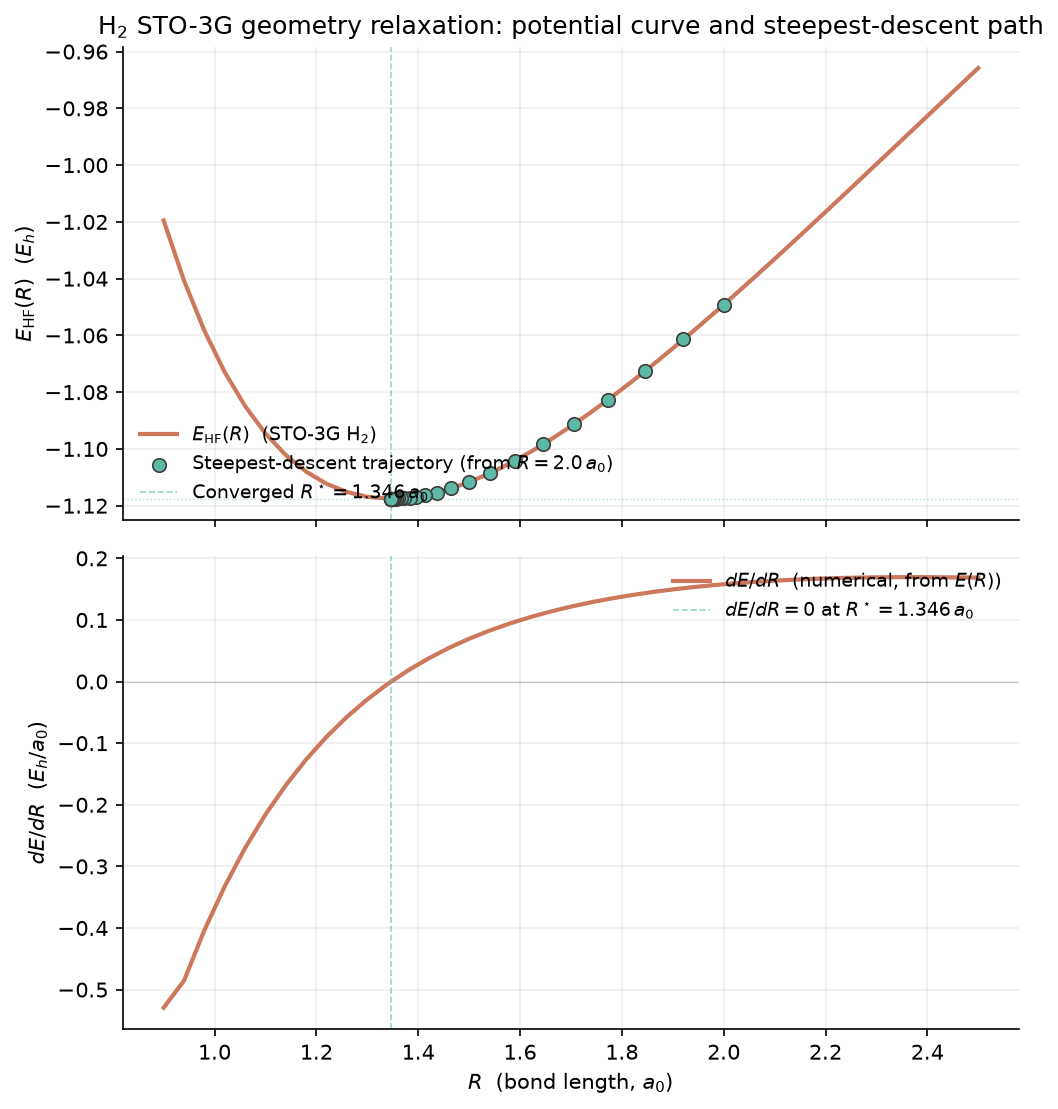
Figure 1. Top: the STO-3G HF potential-energy curve of $\rm H_2$ as a function of bond length, with the steepest- descent trajectory overlaid (red markers). The minimum is at $R^\star \approx 1.346 a_0$ with $E_\text{min} \approx -1.117 E_h$, and the dissociation energy is $D_e \approx 0.079 E_h \approx 2.15$ eV. Bottom: the gradient $dE/dR$ (the “force on the bond”) plotted against $R$. The force vanishes at the minimum and is linear in $(R - R^\star)$ for small displacements, as expected from the harmonic approximation $E(R) \approx E_\text{min} + \tfrac{1}{2} k (R - R^\star)^2$ with $k = d^2 E/dR^2 \approx 0.4\,E_h/a_0^2$.

The full source is at dft_notes/python_codes/chapter_09/01-h2-bond-relaxation.py. The main pieces are the integral routines (inherited from chapter 06), the SCF loop, the gradient evaluation by central differences, the HF force evaluation by grid quadrature on the SCF density, and the steepest-descent step. No external dependencies beyond numpy, scipy, and ‘matplotlib’ (with ‘Agg’ for headless plotting).

9.11 Diagram: the geometry-optimisation loop

%%{init: {'flowchart': {'htmlLabels': true, 'curve': 'basis'}}}%%
graph TD
  R0["Initial geometry<br/>R(0)"] --> E0["SCF at R(0)<br/>(chapter 04)"]
  E0 --> E1["E(R(0)), rho(r), P"]
  E1 --> F1["Compute forces<br/>F_I = -dE/dR_I<br/>Hellmann-Feynman +<br/>Pulay (ch09 §9.3)"]
  F1 --> CK{"Converged?<br/>|F_I| < F_tol<br/>and |dE| < E_tol"}
  CK -->|yes| DONE["Equilibrium geometry<br/>R*, E*"]
  CK -->|no| ST["Choose step<br/>direction p(k)"]
  ST --> SD["Steepest descent<br/>p = -F<br/>(simple)"]
  ST --> NR["Newton<br/>p = -H^-1 F<br/>(quadratic)"]
  ST --> BF["BFGS / LBFGS<br/>(quasi-Newton,<br/>super-linear)"]
  SD --> LS["Line search<br/>alpha_k"]
  NR --> TR["Trust region<br/>|p| <= Delta_k"]
  BF --> TR
  LS --> RNEW["R(k+1) = R(k) +<br/>alpha_k p(k)"]
  TR --> RNEW
  RNEW --> E0

The top half of the diagram (from ‘R(0)’ to ‘F_I) is the *single-point* force evaluation: run an SCF, compute the energy, compute the forces. The bottom half is the *outer loop*: choose a step direction, choose a step length, update the geometry, run the next SCF. The two halves are the same SCF + force code; they differ only in who is calling whom.

9.12 Problems

9.13 What we left out

This chapter covered the analytical gradient in DFT and the geometry-optimisation loop that uses it. Some of the obvious follow-ups we did not cover:

• Ab-initio molecular dynamics (AIMD). Once the forces are in hand, the classical equations of motion $M_I \ddot{\mathbf R}_I = \mathbf F_I$ can be integrated forward in time to generate a trajectory of the nuclei. Born–Oppenheimer AIMD re-runs the SCF at every time step; Car–Parrinello AIMD propagates the orbitals alongside the nuclei with a fictitious electronic mass. Both are sub-fields in their own right; see Marx & Hutter, Ab Initio Molecular Dynamics, Cambridge (2009). The forces in this chapter are exactly the ones used in AIMD; the only new ingredient is the integrator (Verlet, velocity-Verlet, Nose–Hoover thermostat, etc.).
• Nudged elastic band (NEB). To find a transition state between two minima, one relaxes a chain of geometries (the “images”) connected by springs, with the spring force projected out of the perpendicular component and the true force projected out of the tangential component. The resulting “nudged” force is the gradient of the NEB functional, and the algorithm is the same BFGS / LBFGS machinery applied to a chain of geometries. See Henkelman & Jónsson, J. Chem. Phys. 113, 9978 (2000).
• Dimer method and growing-string method. When only one minimum and a rough idea of the transition state are known, the dimer method rotates a pair of geometries about their midpoint to find the lowest-curvature direction without the need for a full Hessian. The growing-string method grows the chain of images from both ends.
• Transition-state search (nudged-elastic-band, dimer, eigenvector-following, gentlest-ascent dynamics). All of these require a Hessian (or a Hessian-vector product) at the saddle point; the most popular algorithm in production is the Baker–Chan version of eigenvector following, which climbs the lowest-eigenvalue mode of the Hessian while minimising in the orthogonal complement.
• Internal coordinates (Z-matrix, redundant internals). The Cartesian-coordinate description is wasteful for the small vibrations of a molecule: the natural coordinates are bond stretches, angle bends, and dihedral torsions. The Baker–Hubbard transformation from Cartesians to internal coordinates accelerates convergence by 5–10x for typical organic molecules, and is the default in Gaussian’s Berny optimiser and in the ORCA geometry-optimisation module.
• Constrained optimisation. Fixing some degrees of freedom (e.g. the bond length of a reaction coordinate) and optimising the rest is the basis of relaxed scans and of many constrained-MD techniques. The standard tool is the method of Lagrange multipliers, with the constraint gradient added to the force.
• Optimisation in delocalised internal coordinates. The Pulay–Baker approach (Pulay & Fogarasi, 1992) uses delocalised internals that are invariant under symmetry operations of the molecule, with a B-matrix that maps from internal to Cartesian space. This is the gold standard for difficult optimisations (transition metal complexes, weakly bound clusters).
• Cell optimisation in non-cubic systems. The stress tensor of §9.9 is for an arbitrary cell. In practice one maintains a minimum basis of cell parameters (3 angles + 3 lengths for a triclinic cell; fewer with symmetry), and the optimiser works in that reduced space. The Pulay stress and the non-local pseudopotential stress are the two terms that require the most care in a plane-wave code.
• Symmetry handling. Crystallographic and molecular point-group symmetries can be used to reduce the number of independent coordinates, and the gradient must be symmetrised after every step. The implementation in most codes is to work in the symmetry-adapted basis of irreducible representations.

Next: chapter 10 — phonons and vibrations. The force constants (the Hessian of the BO energy surface) determine the vibrational frequencies of a molecule and the phonon dispersion of a solid; the same analytical-force machinery we have built here is the starting point.