Chapter 12 — Time-Dependent DFT
Ground-state DFT is a static theory: it tells you the energy and the density of a system that has been sitting in one external potential forever. Time-dependent DFT is its dynamical extension: it tells you what happens when you shake the potential, and what the system absorbs when you shine light on it.
Up to chapter 11 every calculation we have done is for a system in its time-independent ground state. Real chemistry, however, is dynamical. A dye molecule absorbs a visible photon and jumps to an excited state. A solar cell absorbs a sunbeam and produces a current. A molecule in a strong laser pulse ionises while the field is still on. To handle any of these situations we need a time-dependent generalisation of the Kohn–Sham machinery of chapter 04.
That generalisation is the subject of this chapter. We will, in order: state the Runge–Gross theorem that puts TD-DFT on the same formal footing as ground-state DFT; write down the time-dependent Kohn–Sham equations; discuss the practical time-dependent xc potential (adiabatic LDA, exact exchange, Bethe–Salpeter); derive linear-response TD-DFT and the Casida eigenvalue problem for excitation energies and oscillator strengths; introduce real-time TD-DFT as a non-perturbative alternative; close with a worked example of the absorption spectrum of a two-level system, the chapter’s Mermaid workflow, three graded problems, and an honest list of omissions.
Reading note. This chapter assumes chapters 01–05 and 09. Section 12.7 (Casida) presupposes the response-function language of chapter 09 at the level of knowing what a density-response function is and how it enters a Dyson equation.
12.1 The claim — Runge–Gross (1984)
The headline result of the chapter, due to Erich Runge and Eberhard K. U. Gross (1984), is the time-dependent analogue of Hohenberg–Kohn.
Runge–Gross theorem. Fix a many-body Hamiltonian $\hat H(t) = \hat T + \hat W + \hat V(t)$ with the electron- electron interaction $\hat W$ held fixed and a one-body external potential $v_\text{ext}(\mathbf r, t)$ that is Taylor-expandable about $t = t_0$. Fix an initial many-body state $|\Psi_0\rangle$ at $t_0$. Then the mapping ```mermaid %%{init: {‘flowchart’: {‘htmlLabels’: true, ‘curve’: ‘basis’}}}%% graph LR V[“v_ext(r, t)
(time-dependent
external potential)”] –> SE[“Schrodinger equation
i hbar d/dt |Psi(t)>
= H(t) |Psi(t)>”] PSI0[“Initial state |Psi_0>
at t = t_0”] –> SE SE –> PSI[“|Psi(t)>
(time-dependent
many-body state)”] PSI –> RHO[“rho(r, t)
time-dependent
density”] RHO -.->|”RG:
one-to-one (up to c(t))”| V RHO –> OBS[“Every observable
O(t) = <Psi(t) | O | Psi(t)>
is a functional of
rho(r, t) and |Psi_0>”]
classDef inp fill:#eef0e6,stroke:#3a4031,color:#1c1f17; classDef out fill:#cc785c,stroke:#1c1f17,color:#ffffff; classDef mid fill:#d6dcc8,stroke:#3a4031,color:#1c1f17; class V inp class PSI0 inp class SE mid class PSI mid class RHO mid class OBS out
$$
> \begin{equation}
> \label{eq:ch-12-rg-map}
> v_\text{ext}(\mathbf r, t) \;\longmapsto\; \rho(\mathbf r, t)
> \end{equation> is, for a given $|\Psi_0\rangle$, one-to-one up
> to an additive purely time-dependent function
> $c(t)$.

Concretely: if two external potentials $v_\text{ext}(\mathbf r, t)$
and $v'_\text{ext}(\mathbf r, t)$ differ by more than a purely
time-dependent function $c(t)$ at the initial time $t_0$ — i.e. if
their Taylor coefficients
$\partial_t^k (v_\text{ext} - v'_\text{ext})|_{t_0}$ are not all
equal to a single constant in $\mathbf r$ for some $k$ — then the
resulting time-dependent densities $\rho(\mathbf r, t)$ and
$\rho'(\mathbf r, t)$ are different for $t > t_0$ (for short times
in a neighbourhood of $t_0$).

The proof of \eqref{eq:ch-12-rg-map} is the subject of section
12.3. For now we only need the **consequence**: every observable of
the time-evolving system, evaluated at $t > t_0$, is a functional
of $\rho(\mathbf r, t)$ and $|\Psi_0\rangle$. In particular the
external potential is, up to $c(t)$, a functional of the
time-dependent density. This is the foundation of the rest of the
chapter.

> **Tip.** The "up to $c(t)$" freedom is the time-dependent analogue
> of the "up to a constant" freedom in Hohenberg–Kohn. Adding
> $c(t)$ to $v_\text{ext}$ adds $-c(t)$ to the wavefunction's
> global phase, and leaves every gauge-invariant observable
> unchanged. The density is manifestly gauge-invariant, so the
> freedom drops out of the density-to-potential map.

### 12.1.1 Diagram — the Runge–Gross one-to-one mapping

The Runge–Gross theorem is the *foundation* of TD-DFT: it
guarantees that the time-dependent external potential
$v_\text{ext}(\mathbf r, t)$ is in one-to-one correspondence
with the time-dependent density $\rho(\mathbf r, t)$ (up to a
gauge $c(t)$), given a fixed initial state $|\Psi_0\rangle$.
The diagram below shows the *forward* map (potential → wave
function → density, the natural arrow of the Schrödinger
equation) and the *Runge–Gross* inverse (density → potential,
which is what makes TD-DFT possible).


The **solid** arrows are the forward map — the Schrödinger
equation determines the wave function from the potential, and
the density is the diagonal of the one-body density matrix. The
**dashed** arrow is the Runge–Gross* inverse, which says:
given the *density* $\rho(\mathbf r, t)$ and the initial state
$|\Psi_0\rangle$, the potential $v_\text{ext}(\mathbf r, t)$ is
*uniquely* determined (up to a purely time-dependent function
$c(t)$). This is the time-dependent analogue of the
Hohenberg–Kohn theorem (chapter 04) and is the foundation of
*every* practical TD-DFT calculation: it is what justifies
writing the time-dependent KS potential as a *functional* of
the time-dependent density.

## 12.2 The time-dependent Kohn–Sham equations

The Runge–Gross theorem guarantees the *existence* of a
density-to-potential map. To use it computationally we follow
Kohn and Sham's 1965 strategy (chapter 04, section 4.2) and
introduce an **auxiliary system of non-interacting electrons**
that reproduces the interacting density $\rho(\mathbf r, t)$ at
all times.

### 12.2.1 The auxiliary system

Consider a fictitious system of $N$ non-interacting electrons in
an effective time-dependent potential $v_\text{eff}(\mathbf r, t)$.
Its one-body Hamiltonian is

\label{eq:ch-12-tdks-hamiltonian}
\hat H_s(t) \;=\; -\frac{1}{2}\nabla^2 + v_\text{eff}(\mathbf r, t) ,
$$

and its wavefunction is a single time-dependent Slater determinant
$\Phi_s(t)$ built from $N$ orthonormal orbitals
$\{\phi_i(\mathbf r, t)\}$ that satisfy

$$
\label{eq:ch-12-tdks-orbital}
i\, \frac{\partial}{\partial t}\, \phi_i(\mathbf r, t)
\;=\; \hat H_s(t)\, \phi_i(\mathbf r, t) .
$$

The auxiliary density is

$$
\label{eq:ch-12-tdks-density}
\rho(\mathbf r, t) \;=\; 2 \sum_{i=1}^{N/2} |\phi_i(\mathbf r, t)|^2
$$

for a closed-shell (spin-paired) system, the factor of 2 again
accounting for Kramers-paired spins.

### 12.2.2 The effective potential

Equation \eqref{eq:ch-12-tdks-orbital} becomes useful when we
constrain the auxiliary density \eqref{eq:ch-12-tdks-density} to
*equal* the interacting density. The Runge–Gross theorem then
guarantees that there is a unique (up to $c(t)$) effective
potential $v_\text{eff}(\mathbf r, t)$ that does this. The standard
decomposition of $v_\text{eff}$ mirrors the static case:

$$
\label{eq:ch-12-veff}
v_\text{eff}[\rho](\mathbf r, t)
\;=\; v_\text{ext}(\mathbf r, t)
    + v_\text{H}[\rho_t](\mathbf r, t)
    + v_\text{xc}[\rho_{\le t}](\mathbf r, t) .
$$

Three comments on \eqref{eq:ch-12-veff}:

1. **The Hartree term** $v_\text{H}[\rho_t](\mathbf r, t)$ is the
   *instantaneous* classical Coulomb potential of the density
$$
   \label{eq:ch-12-vh}
   v_\text{H}[\rho](\mathbf r, t)
   \;=\; \int \frac{\rho(\mathbf r', t)}{|\mathbf r - \mathbf r'|}\, d\mathbf r' .
$$
   The subscript $\rho_t$ emphasises that the Hartree potential at
   time $t$ depends on the density at the *same* time $t$ — i.e. it
   is **instantaneous** in the time-dependent sense, even though
   physically there is a retardation built in by the fact that
   $\rho(\mathbf r, t)$ is itself a solution of the time-dependent
   problem.

2. **The xc term** $v_\text{xc}[\rho_{\le t}](\mathbf r, t)$ is in
   principle a functional of the *entire history* of the density
   $\{\rho(\mathbf r, \tau) : \tau \le t\}$ — it is
   **non-local in time**. This is a fundamental difference from
   ground-state DFT, where $v_\text{xc}$ depends on $\rho$ at one
   point in time. Memory effects are part of the exact time-
   dependent xc potential. The vast majority of practical
   calculations use the **adiabatic** approximation
   $v_\text{xc}^\text{ad}[\rho](\mathbf r, t) = v_\text{xc}^\text{gs}[\rho(t)](\mathbf r)$
   — i.e. the static xc potential evaluated on the *instantaneous*
   density — which has no memory. Section 12.4 discusses this
   approximation in detail.

3. **The KS equations are nonlinear.** The effective potential
   \eqref{eq:ch-12-veff} depends on the orbitals (through
   $\rho$), and the orbitals evolve under the effective potential.
   Unlike in linear-response theory (section 12.5) the equations
   are not linear, and closed-form solutions exist only for very
   special $v_\text{ext}$. The numerical work is to time-step
   \eqref{eq:ch-12-tdks-orbital} — see section 12.8. > **Warning.** The "adiabatic" approximation is consistent with
> the static functional only in the limit of *infinitely slow*
> time variation. For a true time-dependent problem, where
> $\rho(\mathbf r, t)$ changes on a time scale comparable to the
> internal electron dynamics, the adiabatic approximation
> introduces uncontrolled errors. We will see this in practice in
> the worked example of section 12.10. ### 12.2.3 The van Leeuwen–Baerends fixed-point formulation

The decomposition \eqref{eq:ch-12-veff} is a *definition* of
$v_\text{xc}$ as "what is left over". A complementary and very
useful reformulation is due to van Leeuwen and Baerends (1994): the
effective potential $v_\text{eff}(\mathbf r, t)$ is the **fixed
point** of an integral equation whose kernel is the inverse of the
non-interacting KS response function. We will not derive this
explicitly (it appears in many standard references) but we use the
idea in section 12.5 when we connect $v_\text{xc}$ to the
exchange–correlation kernel $f_\text{xc}$.

### 12.2.4 The time-dependent KS equations, restated

Putting it all together, the **time-dependent Kohn–Sham equations**
are the coupled system

$$
\label{eq:ch-12-tdks-coupled}
\boxed{
\begin{aligned}
i\, \partial_t \phi_i(\mathbf r, t) &= \Bigl[-\tfrac{1}{2}\nabla^2
   + v_\text{eff}[\rho_t](\mathbf r, t) \Bigr]\, \phi_i(\mathbf r, t) , \\\
\rho(\mathbf r, t) &= 2 \sum_{i=1}^{N/2} |\phi_i(\mathbf r, t)|^2 , \\\
v_\text{eff}[\rho](\mathbf r, t) &=
   v_\text{ext}(\mathbf r, t)
 + v_\text{H}[\rho_t](\mathbf r, t)
 + v_\text{xc}[\rho_{\le t}](\mathbf r, t) .
\end{aligned}
}
$$

The first equation is a (nonlinear) one-body Schrödinger equation;
the second is the density reconstruction from the occupied
orbitals; the third defines the effective potential in terms of
the density. The system is closed: given $v_\text{ext}(\mathbf r,
t)$ and the initial state $\Phi_s(t_0)$, the equations determine
$\rho(\mathbf r, t)$ and $\phi_i(\mathbf r, t)$ for all $t > t_0$.
The only unknown is the **functional form of $v_\text{xc}$**, which
is the subject of section 12.4. ## 12.3 Derivation of the Runge–Gross theorem

This is the section where every step is written out.  The
argument follows Runge and Gross's 1984 paper; the
**action-functional** version uses the reformulation by
Ghosh and Dhara (1988) and van Leeuwen (1998). We give the
fixed-point action derivation, which is the cleanest.

### 12.3.1 The quantum-mechanical action

For a system with Hamiltonian $\hat H(t) = \hat T + \hat W +
\hat V(t)$ and a state $|\Psi(t)\rangle$ that solves the
time-dependent Schrödinger equation
$i\, \partial_t |\Psi(t)\rangle = \hat H(t) |\Psi(t)\rangle$
with initial condition $|\Psi(t_0)\rangle = |\Psi_0\rangle$, the
**quantum-mechanical action functional** is

$$
\label{eq:ch-12-action}
\mathcal A[\Psi]
\;=\; \int_{t_0}^{t_1}
   \Bigl\langle \Psi(t) \Big|
   i\, \partial_t - \hat H(t) \Big| \Psi(t) \rangle \Bigr\rangle\, dt .
$$

The action is **stationary** ($\delta \mathcal A = 0$) at the
physical $|\Psi(t)\rangle$, with fixed endpoints
$|\Psi(t_0)\rangle = |\Psi_0\rangle$ and
$|\Psi(t_1)\rangle = |\Psi_1\rangle$. The proof is a standard
functional variation; expanding
$|\Psi\rangle \to |\Psi\rangle + \epsilon |\delta\Psi\rangle$ and
collecting terms of order $\epsilon$ gives the time-dependent
Schrödinger equation back, with the boundary-condition term
$\langle \delta\Psi(t_1) | \Psi(t_1) \rangle - \langle
\delta\Psi(t_0) | \Psi(t_0) \rangle$ vanishing because the
endpoints are fixed.

### 12.3.2 The Keldysh contour

For a system with a *time-dependent* Hamiltonian, the natural
contour for the time integral is the **Keldysh contour** $\gamma$
that runs from $t_0$ to $t_1$ on the upper branch and back from
$t_1$ to $t_0$ on the lower branch, with $t_0 \to -\infty$ and
$t_1 \to +\infty$ at the end. The reason is that the density
matrix at time $t$ — and hence the action that generates it —
involves both forward and backward propagation in time. Define

$$
\label{eq:ch-12-keldysh-action}
\mathcal A_\gamma[\Psi]
\;=\; \int_\gamma
   \Bigl\langle \Psi(\bar t) \Big|
   i\, \partial_{\bar t} - \hat H(\bar t) \Big| \Psi(\bar t) \rangle \Bigr\rangle\, d\bar t ,
$$

where $\bar t$ parameterises the contour. The integrand on the
upper branch is the same as in \eqref{eq:ch-12-action}; on the
lower branch $\partial_{\bar t} = -\partial_t$, so the sign of
the kinetic term flips. The result is that the action
\eqref{eq:ch-12-keldysh-action} is *real* and stationary at
the physical forward–backward trajectory. The vanishing of
$\delta \mathcal A_\gamma = 0$ for variations with fixed
endpoints at $t_0$ is again equivalent to the time-dependent
Schrödinger equation on each branch.

### 12.3.3 The Runge–Gross action

The Keldysh action \eqref{eq:ch-12-keldysh-action} is a
functional of $|\Psi(t)\rangle$ and of $v_\text{ext}(\mathbf r, t)$.
The first variation with respect to the wavefunction gives the
Schrödinger equation, which we already used. The Runge–Gross
trick is to instead **eliminate** the wavefunction in favour of
the density.

To do this, write the interacting action as

$$
\label{eq:ch-12-rg-action}
\mathcal A_\gamma[v_\text{ext}, \Psi]
\;=\; \mathcal B_\gamma[\Psi]
   - \int_\gamma \int d\mathbf r\,
       \rho_\Psi(\mathbf r, \bar t)\,
       v_\text{ext}(\mathbf r, \bar t) ,
$$

where $\mathcal B_\gamma[\Psi] = \int_\gamma d\bar t\, \langle
\Psi | i\partial_{\bar t} - \hat T - \hat W | \Psi \rangle$ is
the **universal** part (independent of $v_\text{ext}$) and the
second term is the coupling to the external potential,
$\rho_\Psi(\mathbf r, \bar t) = \langle \Psi(\bar t) |
\hat\rho(\mathbf r) | \Psi(\bar t) \rangle$ being the
time-dependent density.

Now define the **density functional**

$$
\label{eq:ch-12-A-density-functional}
\mathcal A_\gamma[v_\text{ext}, \rho]
\;=\; \mathcal B_\gamma[\rho]
   - \int_\gamma \int d\mathbf r\,
       \rho(\mathbf r, \bar t)\,
       v_\text{ext}(\mathbf r, \bar t) ,
$$

where $\mathcal B_\gamma[\rho]$ is the **Levy–Lieb** constrained-
search functional

$$
\label{eq:ch-12-B-rho}
\mathcal B_\gamma[\rho]
\;=\; \min_{\Psi \to \rho}
   \int_\gamma d\bar t\,
   \Bigl\langle \Psi \Big|
   i\partial_{\bar t} - \hat T - \hat W \Big| \Psi \Bigr\rangle ,
$$

with the minimum taken over all $N$-electron states
$|\Psi(\bar t)\rangle$ on the contour whose density equals
$\rho(\mathbf r, \bar t)$ for each $\bar t$ on $\gamma$. (The
constraint is the obvious time-dependent generalisation of the
Levy–Lieb functional of static DFT, [chapter 02](/DFT-notes/dft-notes/chapter-02/),
section 2.4.) For a $v_\text{ext}$-representable density, the
minimum is attained at the physical $|\Psi(\bar t)\rangle$ and
$\mathcal B_\gamma[\rho] = \mathcal B_\gamma[\Psi]$.

### 12.3.4 The Runge–Gross proof

> **Why not an action argument?**  It is tempting to vary the
> Keldysh action $\mathcal B_\gamma[\rho]$ and read off a
> fixed-point equation $\delta\mathcal B_\gamma/\delta\rho =
> v_\text{ext}$.  That route is *circular*: subtracting the two
> fixed-point equations for $v$ and $v'$ presumes that
> $\delta\mathcal B_\gamma/\delta\rho$ is a single-valued
> functional of $\rho$ — which is precisely the invertibility the
> theorem is supposed to establish.  The genuine proof instead
> works directly with the quantum-mechanical equations of motion.

**Setup (Runge & Gross 1984).**  Two external potentials
$v(\mathbf r, t)$ and $v'(\mathbf r, t)$ evolve the *same*
initial state $|\Psi_0\rangle$ and are both expandable in Taylor
series about $t_0$.  Suppose they produce the same density:
$\rho(\mathbf r, t) = \rho'(\mathbf r, t)$ for all $t \ge t_0$.

**Step 1 — equal densities imply equal currents.**  By the
continuity equation $\partial_t\rho + \nabla\cdot\mathbf j = 0$
with identical initial data $\rho(\mathbf r, t_0)$ and
$\mathbf j(\mathbf r, t_0)$ (same $|\Psi_0\rangle$), equal
densities force $\mathbf j = \mathbf j'$ everywhere.

**Step 2 — first equation of motion.**  The Heisenberg equation
for the paramagnetic current gives Newton's law in local form,

$$
\partial_t \mathbf j(\mathbf r, t)
   \;=\; -\rho(\mathbf r, t)\,\nabla v(\mathbf r, t)
        + \mathbf T(\mathbf r, t),
$$

where $\mathbf T$ is built from the kinetic operator and the
state alone.  At $t = t_0$ both systems share $|\Psi_0\rangle$,
so their $\mathbf T$ terms coincide.  Subtracting the two
equations of motion and using $\rho = \rho'$:

$$
\rho(\mathbf r, t_0)\,
\nabla\bigl[v - v'\bigr](\mathbf r, t_0) \;=\; 0 .
$$

On the support of $\rho(\mathbf r, t_0)$ (a $v$-representable
density is positive there by assumption), this forces
$\nabla(v-v')(\mathbf r, t_0) = 0$, i.e.
$v(\mathbf r, t_0) - v'(\mathbf r, t_0) = c_1$, a constant in
$\mathbf r$.

**Step 3 — iterate in time.**  If $c_1 \neq 0$, differentiate
the equation-of-motion mismatch once more in $t$.  The new
terms contain $\partial_t(v-v')(t_0)$ multiplied by known
quantities fixed entirely by $|\Psi_0\rangle$; each order of
the Taylor expansion therefore forces the next coefficient of
$v - v'$ to be a constant.  Analyticity then makes
$v(\mathbf r, t) - v'(\mathbf r, t) = c(t)$ for all $t$: a
purely time-dependent function.

This is the original **Runge–Gross conclusion**: **two
Taylor-expandable potentials that generate the same density from
the same initial state differ by at most a purely time-dependent
constant** — and such a constant changes nothing physical, since
it shifts every orbital by a phase $e^{-i\int c(t)dt}$.

### 12.3.5 The full statement

To make the proof work with the "up to $c(t)$" caveat rather
than "exactly equal", the technical argument needs the
**$v$-representability** of the density on both branches and
the **Taylor-expandability** of the potentials about $t_0$.
The latter is needed because the constraint
$|\Psi(t_0)\rangle = |\Psi_0\rangle$ fixes the initial state,
and the time-evolution operator
$\hat U(t, t_0)$ depends on the *whole* function
$v_\text{ext}(\cdot, t)$, not just on its value at $t_0$. To
show that $v'_\text{ext} - v_\text{ext} = c(t)$ requires
matching the potentials and all their time derivatives at
$t_0$, which is precisely what Taylor-expandability delivers.

The final statement of the Runge–Gross theorem is therefore:

> **Runge–Gross theorem (1984).** Let $v_\text{ext}(\mathbf r,
> t)$ and $v'_\text{ext}(\mathbf r, t)$ be two real-valued
> analytic functions of $t$ in a neighbourhood of $t_0$ for
> which the many-body problem with initial state $|\Psi_0\rangle$
> has a unique solution. Suppose that, for some $k \ge 0$,
$$
> \begin{equation}
> \label{eq:ch-12-rg-condition}
> \left.\frac{\partial^k}{\partial t^k}
>       \big[ v'_\text{ext}(\mathbf r, t) - v_\text{ext}(\mathbf r, t) \big]
> \right|_{t=t_0} \neq \text{const in } \mathbf r .
> \end{equation}
$$
> Then the time-dependent densities produced by the two
> potentials differ infinitesimally close to $t_0$:
> $\rho'(\mathbf r, t) \neq \rho(\mathbf r, t)$ for $t$ in some
> right-neighbourhood of $t_0$.

The "up to a constant" caveat is the $\partial^k/\partial t^k$
piece of the difference being spatially constant — when *all*
the derivatives are spatially constant, the two potentials
differ by $c(t) = v'_\text{ext}(\mathbf r, t) - v_\text{ext}(\mathbf r, t)$
and the densities are equal.

> **Note.** Runge and Gross's original 1984 paper proved the
> theorem for potentials that are analytic in time and for
> systems that are non-degenerate at $t_0$. The "up to a
> constant" caveat was made explicit by van Leeuwen (1998) in
> the action-functional reformulation we have used here. The
> 1994 paper by van Leeuwen and Baerends gives the
> fixed-point equation for $v_\text{eff}$ in terms of the
> non-interacting response, which is the practical route to
> the time-dependent KS system.

## 12.4 The time-dependent xc potential

Equation \eqref{eq:ch-12-veff} hides the only unknown in the
time-dependent KS equations: the **time-dependent xc potential**
$v_\text{xc}[\rho_{\le t}](\mathbf r, t)$. The exact
functional is unknown. Three practical approximations are
described in this section, in increasing order of accuracy and
cost.

### 12.4.1 The adiabatic LDA (ALDA)

The simplest and most-used approximation is the **adiabatic
local-density approximation** (ALDA, sometimes "ALDA" or just
"adiabatic LDA"). It evaluates the static LDA xc potential on
the *instantaneous* density:

$$
\label{eq:ch-12-alda}
v_\text{xc}^\text{ALDA}[\rho](\mathbf r, t)
\;=\; v_\text{xc}^\text{LDA}\big[\rho(\mathbf r, t)\big](\mathbf r) .
$$

In a spin-paired, spin-unpolarised system the LDA xc potential
is the functional derivative of the LDA xc energy,
$v_\text{xc}^\text{LDA}(\mathbf r) = \partial[\rho(\mathbf r)
\varepsilon_\text{xc}(\rho(\mathbf r))]/\partial\rho(\mathbf r)$
evaluated at $\rho = \rho(\mathbf r, t)$. The adiabatic
approximation sets $v_\text{xc}$ to depend *only* on the
density at the *current* time — i.e. it is **memory-free**.

The ALDA is exact in two limits:

1. **Slowly-varying** potentials, where the density has time to
   track the perturbation and the xc kernel acts
   quasi-instantaneously.
2. **Linear response** of the homogeneous electron gas, where
   the ALDA reproduces the exact high-frequency limit of the
   xc kernel $f_\text{xc}(\mathbf q, \omega) \to f_\text{xc}^\text{ALDA}(\mathbf q)$
   as $\omega \to \infty$.

In between, the ALDA has the well-known failure that it misses
the long-range tail of the xc kernel: the derivative
discontinuity and the step structure in finite systems, the
excitonic effects that bind an electron and a hole in solids,
and the polarisation-dependence of the xc kernel in
time-dependent phenomena. We will see some of these failures
in the worked example of section 12.10. The adiabatic **GGA** (adiabatic PBE, etc.) and adiabatic
**hybrid** functionals follow the same pattern, with the static
functional plugged in at the instantaneous density. They do
not introduce any new physics beyond ALDA — they only improve
the *static* xc potential that is being evaluated adiabatically.

> **Tip.** The "adiabatic" label is a physical statement, not a
> technical one. The static LDA, GGA, or hybrid xc potential is
> a *snapshot* functional: it takes one density as input and
> returns one potential. By *adiabatically* evaluating it on
> $\rho(\mathbf r, t)$ we are saying that the xc potential at
> time $t$ depends only on the density at that same time, with
> no memory of how $\rho$ got there. This is correct only when
> the density changes slowly.

### 12.4.2 The exact-exchange (EXX) kernel

The **exact-exchange** (EXX) approximation is the
time-dependent analogue of the hybrid functionals of
[chapter 04](/DFT-notes/dft-notes/chapter-04/) (section
4.5). At the time-dependent level, "exact exchange" means that
the xc kernel $f_\text{xc}(\mathbf r, \mathbf r', t - t')$ is
approximated by the **Fock exchange kernel** of the KS
orbitals:

$$
\label{eq:ch-12-exx-kernel}
f_\text{x}^\text{EXX}(\mathbf r, \mathbf r', t - t')
\;=\; -\frac{1}{2} \sum_{\sigma}
   \frac{|\gamma_s(\mathbf r, \mathbf r'; t, t')|^2}
        {|\mathbf r - \mathbf r'|\, \rho(\mathbf r, t)\, \rho(\mathbf r', t')}\, \delta(t - t') .
$$

(The $\delta(t - t')$ enforces the *adiabatic* approximation;
EXX is, in practice, almost always used adiabatically.) The
"$\frac{1}{2}$" is the same exchange factor as in Hartree–Fock;
the sum runs over the Kramers spin pair; and
$\gamma_s(\mathbf r, \mathbf r'; t, t')$ is the one-body
density matrix of the KS Slater determinant.

The EXX kernel captures the **long-range $-\!1/r$ tail** that
ALDA misses, and the related derivative discontinuity in the
xc potential at particle-number changes. In practice EXX is
implemented by the same frequency-dependent kernel that the
Bethe–Salpeter equation uses (next subsection); a fully
time-dependent EXX code is rare.

The practical cost of EXX scales as $\mathcal O(K^4)$ in a
Gaussian basis (the same as HF exchange), making it 1–2 orders
of magnitude more expensive than ALDA but still much cheaper
than BSE.

### 12.4.3 The Bethe–Salpeter equation (BSE)

The **Bethe–Salpeter equation** (BSE) is not, strictly, a
time-dependent xc *functional*: it is a four-point equation for
the two-particle Green's function $L(1, 2; 3, 4)$ that lives at
a higher level of the many-body hierarchy. But it is the
standard *bridge* between TD-DFT and a description of two-
particle excitations (excitons), and we include it here for
completeness.

The BSE for the two-particle correlation function
$L(1, 2; 3, 4)$ is

$$
\label{eq:ch-12-bse}
L(1, 2; 3, 4)
\;=\; L_0(1, 2; 3, 4)
   + \int d5\, d6\, d7\, d8\,
   L_0(1, 5; 3, 7)\,
   K(5, 6; 7, 8)\,
   L(8, 6; 2, 4) ,
$$

where $L_0$ is the non-interacting two-particle propagator
(built from the KS orbitals and quasiparticle energies), and
$K$ is the **Bethe–Salpeter kernel**. In the standard
approximation $K = K^x + K^\text{direct}$ where
$K^x = \bar v$ is the **exchange** kernel (the *bare*
Coulomb interaction — repulsive) and $K^\text{direct} = -W$
is the **direct** (correlation) kernel — the *statically
screened* Coulomb interaction $W$, entered with a minus sign
and therefore **attractive** between the excited electron and
the hole it left behind.

The BSE captures the **electron–hole interaction** that binds
an exciton in a semiconductor. Standard ALDA TD-DFT misses
this entirely because the ALDA xc kernel is short-ranged; BSE
recovers it because the BSE kernel contains the long-range
Coulomb interaction. The price is that the BSE is an
$\mathcal O(N^6)$ eigenvalue problem in a basis of single-
particle transitions (or $\mathcal O(N^4)$ in storage for the
matrix), where $N$ is the number of KS states. We do not
derive the BSE here — the standard references are
Strinati (1988), Rohlfing and Louie (2000), and the
review by Onida, Reining, and Rubio (2002).

> **Note.** The hierarchy of TD-DFT, BSE, and the GW approximation
> (a related many-body method) is intricate. ALDA TD-DFT is a
> long-wave-approximation limit of BSE. EXX TD-DFT is the
> adiabatic limit of BSE with $K = K^x$ (the exchange kernel
> only, no direct term). Full BSE with the screened-Coulomb
> kernel is the most accurate and the most expensive of the
> three. We summarise the relationships in section 12.11. ## 12.5 Linear-response TD-DFT (TD-DFRT)

The exact time-dependent KS equations are nonlinear. The
**linear-response** regime — the response to a *weak*
perturbation — is far more tractable and is the workhorse of
practical TD-DFT for excitation spectra.

### 12.5.1 The density-density response function

For a system in its ground state $|\Psi_0\rangle$, the response
of the density to a weak external perturbation
$\delta v_\text{ext}(\mathbf r, t)$ is described by the
**density-density response function** $\chi$:

$$
\label{eq:ch-12-chi-def}
\delta\rho(\mathbf r, t) \;=\;
\int dt' \int d\mathbf r'\,
   \chi(\mathbf r, t; \mathbf r', t')\,
   \delta v_\text{ext}(\mathbf r', t') .
$$

In a time-translation-invariant system the response depends
only on $t - t'$, and the Fourier transform with respect to
$\tau = t - t'$ gives the **frequency-dependent** response
function $\chi(\mathbf r, \mathbf r'; \omega)$:

$$
\label{eq:ch-12-chi-fourier}
\delta\rho(\mathbf r, \omega) \;=\;
\int d\mathbf r'\,
   \chi(\mathbf r, \mathbf r'; \omega)\,
   \delta v_\text{ext}(\mathbf r', \omega) .
$$

The poles of $\chi(\mathbf r, \mathbf r'; \omega)$ as a
function of $\omega$ give the **neutral excitation energies**
of the interacting system. The residues at the poles give the
**oscillator strengths** — the same quantities that enter
Fermi's golden rule for photon absorption. This is the
content of section 12.6. ### 12.5.2 The KS response function

The non-interacting KS system has its own response function,
$\chi_s$, which describes how the KS density responds to a
weak perturbation of the KS effective potential:

$$
\label{eq:ch-12-chi-s-def}
\delta\rho_s(\mathbf r, \omega) \;=\;
\int d\mathbf r'\,
   \chi_s(\mathbf r, \mathbf r'; \omega)\,
   \delta v_\text{eff}(\mathbf r', \omega) .
$$

In a basis of KS orbitals the KS response function is
**independent** of the time-dependent xc potential; it depends
only on the KS orbitals and eigenvalues. Its Lehmann
representation is

$$
\label{eq:ch-12-chi-s-lehmann}
\chi_s(\mathbf r, \mathbf r'; \omega) \;=\;
2 \sum_{i}^\text{occ} \sum_{a}^\text{virt}
   \frac{\phi_i^*(\mathbf r)\, \phi_a(\mathbf r)\,
         \phi_a^*(\mathbf r')\, \phi_i(\mathbf r')}
        {\omega - (\varepsilon_a - \varepsilon_i) + i\eta}
   \;-\; \text{c.c.}(\omega \to -\omega) .
$$

The "2" is again the Kramers spin-pairing factor; the sum is
over occupied ($i$) and virtual ($a$) KS orbitals; and the
"c.c." term subtracts the same expression with $\omega$ sent
to $-\omega$ to enforce the proper-particle / hole
asymmetry. The infinitesimal $i\eta$ with $\eta \to 0^+$ picks
out the retarded response function.

The poles of $\chi_s$ sit at the **KS single-particle
excitation energies** $\varepsilon_a - \varepsilon_i$ —
*not* at the true many-body excitation energies. The whole
point of the Dyson equation (next subsection) is to dress
$\chi_s$ with the electron–electron interaction and shift the
poles to the correct many-body positions.

### 12.5.3 The Dyson equation

The full interacting response function $\chi$ is connected to
the KS response $\chi_s$ by the **Dyson equation**

$$
\label{eq:ch-12-dyson}
\boxed{
\chi(\mathbf r, \mathbf r'; \omega) \;=\;
\chi_s(\mathbf r, \mathbf r'; \omega)
   + \int d\mathbf r''\, d\mathbf r'''\,
   \chi_s(\mathbf r, \mathbf r''; \omega)\,
   \Bigl[ v_\text{H}(\mathbf r'', \mathbf r''')
        + f_\text{xc}(\mathbf r'', \mathbf r''', \omega) \Bigr]\,
   \chi(\mathbf r''', \mathbf r'; \omega) .
}
$$

The kernel is the sum of the **Hartree kernel**
$v_\text{H}(\mathbf r, \mathbf r') = 1/|\mathbf r - \mathbf r'|$
and the **exchange–correlation kernel**

$$
\label{eq:ch-12-fxc}
f_\text{xc}(\mathbf r, \mathbf r', \omega) \;=\;
\frac{\delta v_\text{xc}(\mathbf r, \omega)}
     {\delta \rho(\mathbf r', \omega)} ,
$$

which is the *functional derivative* of the time-dependent
xc potential with respect to the density, evaluated on the
frequency-diagonal piece of the response. The frequency
dependence of $f_\text{xc}$ is the memory effect: the xc
potential at frequency $\omega$ depends on the density at
all frequencies via $f_\text{xc}(\omega)$, and the Dyson
equation couples these through $\chi_s$ (which already
contains the orbital energy denominators).

**Derivation of the Dyson equation.**  The KS density must
equal the interacting density: $\delta\rho = \delta\rho_s$.
The perturbation that the *electrons* actually feel, however,
is not the bare $\delta v_\text{ext}$ but the *self-consistent*
$\delta v_\text{eff}$:

$$
\label{eq:ch-12-veff-response}
\delta v_\text{eff}(\mathbf r, \omega)
\;=\; \delta v_\text{ext}(\mathbf r, \omega)
   + \int d\mathbf r'\,
       v_\text{H}(\mathbf r, \mathbf r')\,
       \delta\rho(\mathbf r', \omega)
   + \int d\mathbf r'\,
       f_\text{xc}(\mathbf r, \mathbf r'; \omega)\,
       \delta\rho(\mathbf r', \omega) .
$$

Substitute into \eqref{eq:ch-12-chi-s-def} and use
$\delta\rho = \delta\rho_s$:

$$
\begin{align}
\delta\rho(\mathbf r, \omega)
&= \int d\mathbf r'\,
     \chi_s(\mathbf r, \mathbf r'; \omega)\,
     \Bigl[ \delta v_\text{ext}(\mathbf r', \omega)
           + \int d\mathbf r''\,
              v_H(\mathbf r', \mathbf r'')\,
              \delta\rho(\mathbf r'', \omega)
           + \int d\mathbf r''\,
              f_\text{xc}(\mathbf r', \mathbf r''; \omega)\,
              \delta\rho(\mathbf r'', \omega) \Bigr] .
\end{align}
$$

Use \eqref{eq:ch-12-chi-fourier} to replace
$\delta v_\text{ext}$ with $\delta\rho$ on the right-hand
side, and rearrange:

$$
\begin{align}
\delta\rho(\mathbf r, \omega)
&= \int d\mathbf r'\,
     \chi_s(\mathbf r, \mathbf r'; \omega)\,
     \delta v_\text{ext}(\mathbf r', \omega) \\\
&\quad + \int d\mathbf r'\, d\mathbf r''\,
     \chi_s(\mathbf r, \mathbf r'; \omega)\,
     \Bigl[ v_H(\mathbf r', \mathbf r'')
          + f_\text{xc}(\mathbf r', \mathbf r''; \omega) \Bigr]\,
     \delta\rho(\mathbf r'', \omega) .
\end{align}
$$

Identifying the first term on the right-hand side as
$\int \chi_s\, \delta v_\text{ext}$ and the rest as the
integral operator applied to $\delta\rho$, we recognise the
linear integral equation for $\chi$, with $\delta v_\text{ext}$
as the inhomogeneous source. Reading off the kernel of the
equation gives \eqref{eq:ch-12-dyson}.

> **Note.** The Dyson equation \eqref{eq:ch-12-dyson} is the
> time-dependent analogue of the static Dyson equation
> $G = G_0 + G_0 \Sigma G$ of many-body theory. In the
> language of the previous chapter, $\chi$ plays the role of
> the full Green's function $G$, $\chi_s$ the role of $G_0$,
> and $v_H + f_\text{xc}$ the role of the self-energy
> $\Sigma$. The KS orbitals take the place of the
> mean-field orbitals of the Hartree–Fock starting point.

### 12.5.4 The two-particle-like structure

Although \eqref{eq:ch-12-dyson} is a two-point function
equation, it has a **four-index matrix** structure when
discretised. In a basis of $K$ spatial functions,
$\chi(\mathbf r, \mathbf r'; \omega)$ becomes a $K \times K$
matrix $\chi(\omega)$, and the integral
$\int d\mathbf r''\, d\mathbf r'''$ becomes matrix
multiplication:

$$
\label{eq:ch-12-dyson-matrix}
\boldsymbol\chi(\omega) \;=\;
\boldsymbol\chi_s(\omega)
   + \boldsymbol\chi_s(\omega)\,
     \Bigl[ \mathbf v_H + \mathbf f_\text{xc}(\omega) \Bigr]\,
     \boldsymbol\chi(\omega) .
$$

This is a $K \times K$ matrix equation for the $K \times K$
matrix $\boldsymbol\chi(\omega)$. Solving it for $\boldsymbol\chi$
at each frequency — or, more efficiently, finding its poles
and residues — is the practical work of linear-response
TD-DFT.

## 12.6 Excitations

The poles of the response function $\chi(\mathbf r, \mathbf r';
\omega)$ are the **neutral excitation energies** of the system.
To see this, write the Dyson equation \eqref{eq:ch-12-dyson-matrix}
in operator form as

$$
\label{eq:ch-12-chi-resolvent}
\boldsymbol\chi(\omega) \;=\;
\Bigl[ \mathbf 1 - \boldsymbol\chi_s(\omega)\,
     \Bigl( \mathbf v_H + \mathbf f_\text{xc}(\omega) \Bigr)
\Bigr]^{-1}\, \boldsymbol\chi_s(\omega) .
$$

The poles of $\boldsymbol\chi(\omega)$ are the frequencies
$\omega_I$ at which the bracketed matrix is singular, i.e. at
which

$$
\label{eq:ch-12-pole-equation}
\det\Bigl[ \mathbf 1 - \boldsymbol\chi_s(\omega_I)\,
                \Bigl( \mathbf v_H + \mathbf f_\text{xc}(\omega_I) \Bigr)
       \Bigr] \;=\; 0 .
$$

At such a frequency the response is *infinite* for a finite
perturbation — i.e. a *resonance* of the system. The
$\omega_I$ for which the response blows up are the **excitation
energies**.

### 12.6.1 Oscillator strengths

The **oscillator strength** $f_I$ of an excitation at energy
$\omega_I$ is the residue of $\boldsymbol\chi$ at the pole
$\omega = \omega_I$. It measures the strength of the
excitation's coupling to a uniform electric field (in the
dipole approximation) and is directly comparable to
experimental absorption cross-sections via the relation

$$
\label{eq:ch-12-oscillator-strength}
\sigma(\omega) \;=\; \frac{2\pi^2}{c} \sum_I f_I\, \delta(\omega - \omega_I) ,
$$

where $\sigma(\omega)$ is the cross-section for absorption of
a photon of energy $\omega$.

For a closed-shell, dipole-allowed excitation the oscillator
strength in the dipole-length gauge is

$$
\label{eq:ch-12-fI}
f_I \;=\; \frac{2\, m\, \omega_I}{3\hbar}\,
   \sum_{\alpha = x, y, z}
   \Bigl| \langle \Psi_I | \hat r_\alpha | \Psi_0 \rangle \Bigr|^2 ,
$$

with $\Psi_0$ the ground state, $\Psi_I$ the excited state, and
$\hat r_\alpha$ the dipole operator in the $\alpha$ direction.
The factor 2 in front is the standard convention in the
*length* gauge; the velocity gauge uses
$|\langle \Psi_I | \hat p_\alpha | \Psi_0 \rangle|^2$ instead.

> **Tip.** The oscillator strength is dimensionless. The
> "Thomas–Reiche–Kuhn sum rule" (problem 1) says that the sum
> of all oscillator strengths of a one-electron system is
> exactly 1. For a many-electron system the sum is $N$, the
> number of electrons. The sum rule is the most important
> sanity check on any computed spectrum.

## 12.7 The Casida formulation

The most widely-used form of the linear-response TD-DFT
eigenvalue problem is due to **Mark Casida** (1995, 1996). It
reduces the search for the poles of $\chi$ to a single
generalised matrix eigenvalue equation of dimension
$N_\text{trans} = N_\text{occ}\, N_\text{virt}$, where
$N_\text{occ}$ and $N_\text{virt}$ are the number of occupied
and virtual KS orbitals.

### 12.7.1 The Casida matrix

The Casida formulation works in the space of single-particle
excitations $|i \to a\rangle$ (one occupied orbital $i$, one
virtual orbital $a$). In this basis the Dyson equation
\eqref{eq:ch-12-dyson} reduces to a matrix equation.

The derivation below is the original Casida (1995) form (Casida,
"Time-dependent density functional response theory for molecules",
in *Recent Advances in Density Functional Methods*, ed. D. P.
Chong, World Scientific, 1995, pp. 155-192; equation numbers
below are from the printed proceedings, pp. 165-168), with the
modern $X$/$Y$ matrix form that Petersilka, Gossmann & Gross
(PRL **76**, 1212, 1996, Eqs. (8)-(9)) re-derived in a slightly
different way.

**Step 1 — the single-particle transition density.** Define

$$
\label{eq:ch-12-transition-density}
\xi_{ia}(\mathbf r) \;=\; \phi_i^*(\mathbf r)\, \phi_a(\mathbf r) ,
$$

the product of an occupied and a virtual KS orbital. The set
$\{\xi_{ia}\}$ for all pairs $(i, a)$ is the basis in which the
Casida matrix is written. The number of basis functions is
$N_\text{trans} = N_\text{occ}\, N_\text{virt}$ (typically
$10^3$ to $10^7$ for a molecule or solid; the eigenvalue problem
is the bottleneck of linear-response TDDFT).

**Step 2 — the KS response in the transition basis.** The KS
response function \eqref{eq:ch-12-chi-s-lehmann} in this basis is
diagonal (this is the *defining* property of the KS response
function — the KS system has no coupling between different
particle–hole pairs):

$$
\label{eq:ch-12-chi-s-lehmann-basis}
\chi_s(\mathbf r, \mathbf r'; \omega) \;=\;
2 \sum_{ia} \xi_{ia}(\mathbf r)\,
       \Bigl[ (\omega - \omega_{ia} + i\eta)^{-1}
            - (\omega + \omega_{ia} - i\eta)^{-1} \Bigr]\,
       \xi_{ia}^*(\mathbf r') ,
$$

with $\omega_{ia} = \varepsilon_a - \varepsilon_i > 0$ the
KS excitation energy of the transition $i \to a$. The factor 2
is the spin sum (closed shell; for an open-shell system it is
replaced by a $2 \times 2$ spin structure). The $i\eta$ is the
standard Feynman prescription that places the poles in the
lower half of the complex $\omega$ plane (so that the response
is causal).

**Step 3 — the density ansatz in the transition basis.** At a
pole of $\chi$ (i.e. at an excitation energy $\omega = \omega_I$),
the first-order density response has a *resonant* (positive
$\omega$) and an *anti-resonant* (negative $\omega$) component.
Write it as

$$
\label{eq:ch-12-rho-ansatz}
\delta\rho(\mathbf r, \omega_I) \;=\; 2 \sum_{ia}
    \Bigl[ X_{ia}\, \xi_{ia}(\mathbf r)
          + Y_{ia}\, \xi_{ia}(\mathbf r) \Bigr] ,
$$

where $X_{ia}$ and $Y_{ia}$ are the *resonant* and anti-resonant
amplitudes of the $ia$ transition in the eigenstate $I$.
Both are real in the spin-summed, time-reversal-symmetric
case. The factor 2 is again the spin sum.

**Step 4 — the self-consistent effective perturbation.** The
effective potential that drives the KS response is the sum of
the external perturbation and the induced Hartree–xc perturbation
\eqref{eq:ch-12-f-Hxc}:

$$
\label{eq:ch-12-v-eff}
\delta v_\text{eff}(\mathbf r, \omega) \;=\;
   \delta v_\text{ext}(\mathbf r, \omega) + \int\! d\mathbf r'\,
        f_\text{Hxc}(\mathbf r, \mathbf r')\,
        \delta\rho(\mathbf r', \omega) .
$$

At the *pole* of $\chi$, the response diverges for a finite
$\delta v_\text{ext}$, so we drop the source and look for a
self-sustaining $\delta v_\text{eff}$:

$$
\label{eq:ch-12-v-eff-pole}
\delta v_\text{eff}(\mathbf r, \omega_I) \;=\;
   \int\! d\mathbf r'\,
        f_\text{Hxc}(\mathbf r, \mathbf r')\,
        \delta\rho(\mathbf r', \omega_I) .
$$

Project onto the transition basis $\xi_{ia}^*(\mathbf r)$ and
integrate over $\mathbf r$:

$$
\label{eq:ch-12-v-eff-ia}
[\delta v_\text{eff}]_{ia} \;=\;
   \sum_{jb} K_{ia, jb}\, 2\,(X_{jb} + Y_{jb}) ,
$$

where the **coupling matrix** $\mathbf K$ is

$$
\label{eq:ch-12-casida-K}
K_{ia, jb} \;=\;
\iint d\mathbf r\, d\mathbf r'\,
   \xi_{ia}^*(\mathbf r)\,
   \Bigl[ v_H(\mathbf r, \mathbf r') + f_\text{xc}(\mathbf r, \mathbf r') \Bigr]\,
   \xi_{jb}(\mathbf r') .
$$

The factor of 2 in \eqref{eq:ch-12-v-eff-ia} comes from the
spin sum in the density ansatz \eqref{eq:ch-12-rho-ansatz}.

**Step 5 — the KS response in the transition basis.** The KS
response is *linear* in $\delta v_\text{eff}$ and diagonal in
the transition basis:

$$
\label{eq:ch-12-rho-from-vs}
\delta\rho(\mathbf r, \omega) \;=\; \int\! d\mathbf r'\,
    \chi_s(\mathbf r, \mathbf r'; \omega)\,
    \delta v_\text{eff}(\mathbf r', \omega) .
$$

Substituting the Lehmann form \eqref{eq:ch-12-chi-s-lehmann-basis}
for $\chi_s$ and projecting onto $\xi_{ia}^*(\mathbf r)$ gives

$$
\label{eq:ch-12-rho-ia}
2\,(X_{ia} + Y_{ia}) \;=\;
   2\,\Bigl[ g_{ia}(\omega_I) + g_{ia}(-\omega_I) \Bigr]\,
   [\delta v_\text{eff}]_{ia} ,
$$

where we have defined the *single-particle propagator*

$$
\label{eq:ch-12-g-ia}
g_{ia}(\omega) \;=\; \frac{1}{\omega - \omega_{ia} + i\eta} ,
$$

whose value at $\omega = \omega_I$ is the relevant object
because $\omega_I$ is the (unknown) pole frequency. Note that
$g_{ia}(-\omega_I) = 1/(-\omega_I - \omega_{ia})$ is small and
regular; only $g_{ia}(\omega_I)$ carries the pole structure.

**Step 6 — separating the resonant and anti-resonant parts.**
Equation \eqref{eq:ch-12-rho-ia} couples $X_{ia}$ and $Y_{ia}$
together. We *separate* them by multiplying the equation by
$g_{ia}(\omega_I)$ and $g_{ia}(-\omega_I)$ separately and using
the identities $g_{ia}(\omega_I) \cdot (\omega_I - \omega_{ia}) = 1$
and $g_{ia}(-\omega_I) \cdot (-\omega_I - \omega_{ia}) = 1$.

For the *resonant* part: multiply the resonant piece of
\eqref{eq:ch-12-rho-ia} (the piece proportional to $g_{ia}(\omega_I)$)
by $(\omega_I - \omega_{ia})$:

$$
\label{eq:ch-12-X-equation}
X_{ia} \;=\; g_{ia}(\omega_I)\, [\delta v_\text{eff}]_{ia} ,
$$

which gives

$$
\label{eq:ch-12-X-equation-2}
(\omega_I - \omega_{ia})\, X_{ia} \;=\; [\delta v_\text{eff}]_{ia} .
$$

Substituting \eqref{eq:ch-12-v-eff-ia} for $[\delta v_\text{eff}]_{ia}$:

$$
\label{eq:ch-12-X-equation-3}
\omega_I\, X_{ia} \;=\; \omega_{ia}\, X_{ia}
    + 2 \sum_{jb} K_{ia, jb}\, (X_{jb} + Y_{jb}) .
$$

For the *anti-resonant* part: multiply the anti-resonant piece
of \eqref{eq:ch-12-rho-ia} (the piece proportional to
$g_{ia}(-\omega_I)$) by $(-\omega_I - \omega_{ia})$:

$$
\label{eq:ch-12-Y-equation}
(-\omega_I - \omega_{ia})\, Y_{ia} \;=\; [\delta v_\text{eff}]_{ia} .
$$

(The resonant part contributes nothing because $g_{ia}(\omega_I)$
is small compared to $g_{ia}(-\omega_I)$ near the negative
frequency pole.) Substituting \eqref{eq:ch-12-v-eff-ia}:

$$
\label{eq:ch-12-Y-equation-2}
-\omega_I\, Y_{ia} \;=\; \omega_{ia}\, Y_{ia}
    + 2 \sum_{jb} K_{ia, jb}\, (X_{jb} + Y_{jb}) .
$$

(After multiplying out the sign in $(-\omega_I - \omega_{ia}) = -(\omega_I + \omega_{ia})$.)

**Step 7 — the Casida equation in modern form.** Equations
\eqref{eq:ch-12-X-equation-3} and \eqref{eq:ch-12-Y-equation-2}
form a $2N_\text{trans}$-dimensional matrix eigenvalue
problem. Writing it in block-matrix form with the diagonal
of the matrix $\mathbf A$ given by the bare excitation
energies $\omega_{ia}$ and the off-diagonal coupling
given by $\mathbf K$:

$$
\label{eq:ch-12-casida}
\boxed{
\begin{pmatrix}
  \mathbf A & \mathbf B \\\
  \mathbf B & \mathbf A
\end{pmatrix}
\begin{pmatrix} \mathbf X \\\\ \mathbf Y \end{pmatrix}
\;=\; \omega_I\,
\begin{pmatrix}
  \mathbf 1 & \mathbf 0 \\\
  \mathbf 0 & -\mathbf 1
\end{pmatrix}
\begin{pmatrix} \mathbf X \\\\ \mathbf Y \end{pmatrix} .
}
$$

The two blocks $\mathbf A$ and $\mathbf B$ are

$$
\label{eq:ch-12-casida-A}
A_{ia, jb} \;=\; \delta_{ij}\, \delta_{ab}\, \omega_{ia}
                + K_{ia, jb} ,
$$

$$
\label{eq:ch-12-casida-B}
B_{ia, jb} \;=\; K_{ia, jb} ,
$$

i.e. the diagonal is the bare KS excitation energy and the
off-diagonal is the same coupling matrix in both blocks. The
identity matrix $\mathbf 1$ and the minus sign on the lower
right come from the *opposite* sign of the pole in the
anti-resonant equation \eqref{eq:ch-12-Y-equation-2}.

**Step 8 — the $\omega^2$ form (Casida 1995, original).** A
common alternative form is obtained by adding and subtracting
the two halves of the eigenvalue problem. Let
$\mathbf F \equiv \mathbf X + \mathbf Y$ and
$\mathbf G \equiv \mathbf X - \mathbf Y$. Adding and
subtracting the two halves of \eqref{eq:ch-12-casida} gives

$$
(\mathbf A + \mathbf B)\, \mathbf F = \omega_I\, \mathbf G , \tag{12.7.a}
$$
$$
(\mathbf A - \mathbf B)\, \mathbf G = \omega_I\, \mathbf F . \tag{12.7.b}
$$

With $\mathbf A - \mathbf B = \mathrm{diag}(\omega_{ia})$
(the coupling cancels because both $\mathbf A$ and $\mathbf B$
have the same off-diagonal $\mathbf K$) and
$\mathbf A + \mathbf B = \mathrm{diag}(\omega_{ia}) + 2\mathbf K$,
equation \eqref{eq:ch-12-b} gives
$\mathbf G = \omega_I\, \mathrm{diag}(\omega_{ia})^{-1}\, \mathbf F$
componentwise, i.e. $G_{ia} = (\omega_I / \omega_{ia})\, F_{ia}$.
Substituting into \eqref{eq:ch-12-a}:

$$
\Bigl[ \mathrm{diag}(\omega_{ia}) + 2\, \mathbf K \Bigr]\,
       \mathbf F
   \;=\; \omega_I^2\, \mathrm{diag}(\omega_{ia})^{-1}\, \mathbf F ,
$$

and multiplying both sides by $\mathrm{diag}(\omega_{ia})$ from
the *left*:

$$
\label{eq:ch-12-casida-omega2}
\boxed{
\mathrm{diag}(\omega_{ia})\,
\Bigl[ \mathrm{diag}(\omega_{ia}) + 2\, \mathbf K \Bigr]\,
       \mathbf F
   \;=\; \omega_I^2\, \mathbf F ,
}
$$

or, in components,

$$
\label{eq:ch-12-casida-omega2-comp}
\sum_{jb} \Bigl[ \delta_{ij}\delta_{ab}\, \omega_{ia}\, \omega_{jb}
                + 2\, \omega_{ia}\, K_{ia, jb} \Bigr]\,
       F_{jb}
   \;=\; \omega_I^2\, F_{ia} .
$$

With the rescaling $\mathbf F = \mathrm{diag}(\omega_{ia})^{-1/2}\,
\boldsymbol\phi$ and a left multiplication by
$\mathrm{diag}(\omega_{ia})^{-1/2}$, equation
\eqref{eq:ch-12-casida-omega2} becomes the **Casida equation in the
symmetric form** (Casida 1995, Eq. (3.16), p. 168):

$$
\Omega_{ia, jb} \;=\; \delta_{ij}\delta_{ab}\, \omega_{ia}^2
   \;+\; 2\,\sqrt{\omega_{ia}}\; K_{ia, jb}\; \sqrt{\omega_{jb}} ,
$$

which is real-symmetric for closed-shell systems, so the
eigenvalues $\omega_I^2$ are real and non-negative. The
square-root rescaling symmetrises the equation and is the standard
presentation; the unsymmetrised form
\eqref{eq:ch-12-casida-omega2-comp} is what was actually derived
above.

In the **Tamm–Dancoff approximation** (TDA, equivalent to
neglecting the $\mathbf B$ block, i.e. setting $Y_{ia} = 0$),
the equation reduces to the simpler eigenvalue problem

$$
\label{eq:ch-12-casida-TDA}
\mathbf A \mathbf X \;=\; \omega_I\, \mathbf X ,
$$

i.e. $\omega_I X_{ia} = \omega_{ia} X_{ia} + 2 \sum_{jb} K_{ia, jb} X_{jb}$.
The TDA is exact for *single* excitations in the limit of
no coupling between particle–hole pairs (i.e. $\mathbf K = 0$)
and is a good approximation for *single excitations* in
general; it underestimates the oscillator strength of
*double* excitations (which require the $\mathbf Y$ block to
be present).

### 12.7.2 The oscillator strength from the Casida eigenvectors

The dipole oscillator strength of excitation $I$ is

$$
\label{eq:ch-12-casida-f}
f_I \;=\; \frac{2}{3} \sum_{\alpha = x, y, z}
   \Bigl| \sum_{ia} \sqrt{\frac{\omega_{ia}}{\omega_I}}\,
        (X_{ia} + Y_{ia})\,
        \langle \phi_a | \hat r_\alpha | \phi_i \rangle \Bigr|^2 .
$$

The sum runs over all single-particle transitions, weighted
by the eigenvectors $(\mathbf X, \mathbf Y)$ of the
$I$-th eigenvalue of \eqref{eq:ch-12-casida}. The factor
$\sqrt{\omega_{ia}/\omega_I}$ is the standard velocity-gauge
rescaling.

### 12.7.3 The form of the coupling matrix

The kernel in \eqref{eq:ch-12-casida-K} separates into a
**Coulomb** part (the Hartree kernel $v_H$) and an
**xc** part (the kernel $f_\text{xc}$). The Coulomb part
drives the **de-excitation** direction in the Casida matrix
(it appears with a $-$ sign in the full equation, but is
absorbed in the structure of $\mathbf A$, $\mathbf B$); the
xc part is what shifts the KS excitation energies to the
true many-body ones.

In the **ALDA** $f_\text{xc}^\text{ALDA}(\mathbf r) =
d^2[\rho \varepsilon_\text{xc}(\rho)]/d\rho^2$, a
*purely local* kernel. The coupling matrix in this case is
often written in terms of spin densities and the spin-
unpolarised or spin-polarised HEG response. The ALDA is
**frequency-independent** — the kernel $f_\text{xc}$ is a
function of $\mathbf r$ only, not of $\omega$. The BSE kernel
is frequency-dependent (it is built from the dynamically
screened Coulomb interaction $W(\omega)$); the EXX kernel
is non-local in $\mathbf r$ but frequency-independent.

> **Note.** The dimension of the Casida matrix is
> $2\, N_\text{occ}\, N_\text{virt}$. For a small molecule
> with $N_\text{occ} = 5$ and $N_\text{virt} = 50$ this is
> a $500 \times 500$ matrix — easily diagonalised. For a
> solid with $N_\text{occ} = 20$ and $N_\text{virt} = 1000$
> it is $40{,}000 \times 40{,}000$, which demands
> iterative eigensolvers. The Casida equation is the
> practical backbone of production TD-DFT codes (Q-Chem,
> TURBOMOLE, ORCA, NWChem).

### 12.7.4 Diagram — the Casida construction pipeline

The Casida equation is the practical realisation of
linear-response TD-DFT for *excitation spectra*. The pipeline
runs from a *ground-state* calculation (which provides the KS
orbitals and energies) through the *KS response function*
$\chi_s$, the *coupling matrix* $\mathbf K$ (which contains the
electron–electron interaction through the kernel $f_\text{xc}$),
and finally a *matrix eigenvalue problem* whose eigenvalues are
the excitation energies $\omega_I$ and whose eigenvectors
$(\mathbf X, \mathbf Y)$ are the *excitation amplitudes*.

```mermaid
%%{init: {'flowchart': {'htmlLabels': true, 'curve': 'basis'}}}%%
graph TD
  GS["Ground state<br/>phi_i, phi_a, eps_i, eps_a<br/>(chapter 04)"] --> TD["Transition densities<br/>xi_ia(r) = phi_i* phi_a"]
  TD --> CHI["KS response function<br/>chi_s(omega)<br/>(Lehmann representation)"]
  CHI --> KERN{"Choose kernel<br/>f_xc(omega)"}
  KERN -->|"ALDA"| ALDA["f_xc = d^2(rho eps_xc)/drho^2<br/>local, omega-independent"]
  KERN -->|"EXX"| EXX["f_xc^EXX<br/>non-local, omega-independent"]
  KERN -->|"BSE"| BSE["K^x + K^direct<br/>non-local, omega-dependent"]
  ALDA --> K["Coupling matrix<br/>K_ia,jb<br/>(eq. 12.78)"]
  EXX --> K
  BSE --> K
  CHI --> A["Diagonal A_ia,jb<br/>= delta_ij delta_ab omega_ia<br/>+ K_ia,jb"]
  K --> A
  K --> B["Off-diagonal B_ia,jb<br/>= K_ia,jb"]
  A --> EIG["Casida eigenvalue problem<br/>(2 N_occ N_virt) x<br/>(2 N_occ N_virt)"]
  B --> EIG
  EIG --> OMEGA["Excitation energies<br/>omega_I<br/>(eigenvalues)"]
  EIG --> XY["Excitation amplitudes<br/>(X_I, Y_I)"]
  XY --> FOSC["Oscillator strength f_I<br/>(eq. 12.80)"]
  OMEGA --> SPEC["UV/vis absorption<br/>spectrum"]
  FOSC --> SPEC

  classDef inp fill:#eef0e6,stroke:#3a4031,color:#1c1f17;
  classDef step fill:#d6dcc8,stroke:#3a4031,color:#1c1f17;
  classDef out fill:#cc785c,stroke:#1c1f17,color:#ffffff;
  class GS inp
  class TD step
  class CHI step
  class KERN step
  class ALDA step
  class EXX step
  class BSE step
  class K step
  class A step
  class B step
  class EIG step
  class XY step
  class FOSC step
  class OMEGA out
  class SPEC out
The three vertical branches of the diagram converge on the
‘EIG’ box. ‘A’ (top branch) provides the diagonal of the
Casida matrix — it contains the KS excitation energies
$\omega_{ia}$ and is the part that survives the Tamm–Dancoff
approximation (TDA, where ‘B’ is neglected). ‘K’ (middle
branch) is the coupling matrix, computed from the chosen
xc kernel; it is the only branch where the kernel choice
matters. B’ (bottom branch) is the de-excitation amplitude
coupling; it is the same matrix as K’ but appears in the
off-diagonal block of the Casida equation. The single matrix
diagonalisation in EIG’ produces all excitation energies and
amplitudes at once; the spectrum is then constructed by
assigning each $\omega_I$ an oscillator strength $f_I$ from the
corresponding eigenvector $(\mathbf X_I, \mathbf Y_I)$.
12.8 Real-time TD-DFT
The Casida equation gives the linear response. For strong fields, non-perturbative dynamics, or systems driven far from equilibrium, the standard alternative is to time-propagate the time-dependent KS equations \eqref{eq:ch-12-tdks-orbital} directly.
12.8.1 The time-propagation algorithm
The simplest integrator for \eqref{eq:ch-12-tdks-orbital} is the Crank–Nicolson (CN) propagator. For the linear part of the Hamiltonian the CN step is unitary, symplectic, and second-order accurate in the time step $\Delta t$. The nonlinear part of the Hamiltonian (the self-consistent update of $v_\text{eff}$) is handled by a predictor- corrector or by an extrapolation of $v_\text{eff}$ to the mid-point of the time step.
The CN update of the orbital $\phi_i$ from $t_n$ to $t_{n+1} = t_n + \Delta t$ is
\[\label{eq:ch-12-cn} \phi_i(t_{n+1}) \;=\; \frac{\mathbf 1 - i\, \tfrac{\Delta t}{2}\, \hat H_s(t_{n+1/2})} {\mathbf 1 + i\, \tfrac{\Delta t}{2}\, \hat H_s(t_{n+1/2})}\, \phi_i(t_n) .\]The fraction on the right is the Cayley transform of the time-evolution operator $\exp(-i \hat H_s \Delta t)$ and is unitary by construction. In a finite basis ${\chi_\mu}{\mu=1}^K$ the operator $(\mathbf 1 + i\, \tfrac{\Delta t}{2}\, \mathbf H_s)$ is a $K \times K$ matrix, and \eqref{eq:ch-12-cn} is a linear solve per orbital per time step. The cost is dominated by the $\mathcal O(K^2)$ effort to build the density and the $\mathcal O(K^2)$ for the matrix-solve — total cost $\mathcal O(N\text{steps}\, K^2)$ per orbital.
The time step is bounded by the highest KS orbital energy included in the propagation. For a typical GGA calculation with a plane-wave cutoff $E_\text{cut} = 30\,E_h$, the smallest time step for stable CN propagation is $\Delta t \lesssim 0.05\,E_h^{-1} \approx 1.2 \times 10^{-3}\,\text{fs}$. A typical UV/vis absorption spectrum requires $T \sim 30\,E_h^{-1} \approx 0.7\,\text{fs}$ of propagation, so $\sim 600$ time steps are needed.
12.8.2 The dipole moment and the spectrum
Once the orbitals have been propagated, the time-dependent dipole moment is
\[\label{eq:ch-12-dipole} \boldsymbol\mu(t) \;=\; \int \rho(\mathbf r, t)\, \mathbf r\, d\mathbf r \;=\; 2 \sum_{i=1}^{N/2} \langle \phi_i(t) | \hat{\mathbf r} | \phi_i(t) \rangle .\]The Fourier transform of $\boldsymbol\mu(t)$ gives the frequency-dependent polarisability $\alpha(\omega)$ and, via the optical theorem, the absorption spectrum:
\[\label{eq:ch-12-spectra-from-dipole} \alpha(\omega) \;\propto\; \int_0^T \boldsymbol\mu(t)\, e^{-i\omega t}\, dt .\]In practice the Fourier transform of a finite-length time series produces sidelobes that obscure the spectrum. The fix is to multiply $\boldsymbol\mu(t)$ by a smooth window function (Hann, Gaussian, exponential damping) before the transform. The damping constant $\eta$ broadens the spectral lines by $\sim \eta$ and gives a finite total propagation time $T = 2\pi/\eta$ the spectral resolution $\Delta\omega \sim 1/T$. There is a trade-off: long propagation gives sharp lines but expensive runs; short propagation gives broad lines but cheap runs.
Tip. The choice of the initial perturbation is one of the few knobs in real-time TD-DFT. A common choice is a delta-function kick in the external potential, $\delta v_\text{ext}(\mathbf r, t) = -k\, \hat z\, \delta(t)$, which excites all dipole-allowed transitions at once. An alternative is a short, finite-width pulse shaped to cover a specific frequency window; this is more efficient for narrow spectral regions. The worked example in section 12.10 uses a delta kick.
12.8.3 The Ehrenfest and surface-hopping extensions
For coupled electron–ion dynamics, the time-dependent KS equations can be coupled to classical nuclear motion via the Ehrenfest mean-field force (the gradient of the time-dependent KS energy at fixed $\rho$), or to surface-hopping trajectories that stochastically branch between adiabatic potential energy surfaces. The Ehrenfest–TDDFT method is the workhorse of ab initio molecular dynamics with electronic excitations; we will not derive the surface-hopping machinery here (it is covered in the molecular-dynamics chapters of the literature).
12.8.4 Diagram — the real-time TD-DFT propagation loop
Real-time TD-DFT propagates the time-dependent KS orbitals forward in time, monitors the time-dependent dipole moment, and extracts the absorption spectrum by Fourier transform. The diagram below shows the propagation loop (top half) and the post-processing chain (bottom half).
%%{init: {'flowchart': {'htmlLabels': true, 'curve': 'basis'}}}%%
graph TD
  GS["Ground state<br/>phi_i(0) = phi_i^GS<br/>(chapter 04)"] --> KICK["Apply perturbation<br/>delta-kick delta v = -k.r delta(t)<br/>or short pulse"]
  KICK --> PHI0["phi_i(t_0+) = phi_i(0)<br/>(kick in v_ext only)"]
  PHI0 --> LOOP["t = t_0, t_0+dt, t_0+2dt, ..."]
  LOOP --> CN["Crank-Nicolson step<br/>phi_i(t+dt) =<br/>(1 - i dt/2 H)/(1 + i dt/2 H) phi_i(t)"]
  CN --> VEFF["Build rho(r, t)<br/>and v_eff[rho](r, t)"]
  VEFF --> CK{"t < T_max?"}
  CK -->|yes| LOOP
  CK -->|no| DONE["Orbital trajectory<br/>phi_i(t), 0 <= t <= T_max"]
  DONE --> MU["Dipole moment<br/>mu(t) = int rho r dr<br/>(eq. 12.97)"]
  MU --> WIN["Multiply by window<br/>(Hann / Gaussian)<br/>suppresses FFT sidelobes"]
  WIN --> FFT["Fourier transform<br/>alpha(omega) = int mu(t) e^{-i omega t} dt"]
  FFT --> SPEC["Absorption spectrum<br/>sigma(omega) ~<br/>omega Im alpha(omega)"]

  classDef inp fill:#eef0e6,stroke:#3a4031,color:#1c1f17;
  classDef prop fill:#d6dcc8,stroke:#3a4031,color:#1c1f17;
  classDef out fill:#cc785c,stroke:#1c1f17,color:#ffffff;
  class GS inp
  class KICK inp
  class PHI0 inp
  class LOOP prop
  class CN prop
  class VEFF prop
  class CK prop
  class DONE out
  class MU out
  class WIN out
  class FFT out
  class SPEC out
The inner loop (‘LOOP’ → ‘CN’ → ‘VEFF’ → ‘CK) is the
propagator: at every time step, the Crank–Nicolson update
rotates each orbital by the Cayley transform of $\hat H_s$,
then a new density and effective potential are built. The
cost per step is $\mathcal O(K^2)$ per orbital (the matrix
solve) plus $\mathcal O(K^2)$ for the density build — total
$\mathcal O(N_\text{steps} N_\text{orb} K^2)$ for the whole
trajectory. The **post-processing** chain ('MU' → 'WIN' → FFT'
→ SPEC`) takes the trajectory and extracts the absorption
spectrum in a single Fourier transform, after windowing to
suppress spectral leakage.
12.12 Applications
Real chemistry and materials science is full of time-dependent phenomena; TD-DFT has carved out a sizeable niche in each. We give a one-line summary of the most common applications; the references are at the end of the section.
- UV/vis absorption spectra. The most common TD-DFT application. The Casida equation is solved for $N_\text{states} \sim 30$–$50$ excited states; the oscillator strengths $f_I$ are plotted against the excitation energies $\omega_I$ and compared with experiment. The accuracy of ALDA TD-DFT is typically $\sim 0.3$ eV for valence excitations of organic molecules; range-separated hybrids (CAM-B3LYP, $\omega$B97X) push this to $\sim 0.2$ eV. Rydberg and charge-transfer excitations remain hard for ALDA — they need a long-range-corrected functional or BSE.
- Excited-state geometries. Optimising the geometry of an excited state requires the gradient of the excited-state energy with respect to nuclear coordinates. In TD-DFT this is the gradient of the Casida eigenvalue $\omega_I$ with respect to the Hamiltonian; the calculation is more involved than the ground-state gradient of chapter 09 but is implemented in production codes. The result gives the equilibrium geometry of the excited state and the adiabatic excitation energy $E_I^\text{ad} = E(\mathbf R_I^) - E(\mathbf R_0^)$.
- Excited-state dynamics. The time-dependent KS equations are propagated together with classical nuclear dynamics; the result is a trajectory in configuration space along which the system decays from the Franck–Condon region to the ground state via non-adiabatic transitions at conical intersections. The Ehrenfest and surface-hopping methods are the two main schemes. The non-adiabatic couplings are computed from the time-dependent KS orbitals.
- Optical response of solids. The macroscopic dielectric function $\epsilon_M(\omega)$ of a periodic solid is obtained from the Casida equation in the Bloch basis, with the momentum operator $\hat{\mathbf p}$ providing the dipole coupling. The resulting spectrum has the same role in linear optics that the ground- state band structure has for static properties.
- Strong-field and attosecond phenomena. Real-time TD-DFT with intense laser pulses ($I \gtrsim 10^{13}$ W/cm²) describes tunnel ionisation, high-harmonic generation, and charge migration in molecules. These phenomena are highly non-perturbative and the linear-response Casida equation does not apply.
- Electronic stopping and warm dense matter. When a swift ion traverses a material, the electronic subsystem is driven far from equilibrium. Real-time TD-DFT in a supercell captures the energy deposition rate and the time-dependent electron distribution.
- Singlet fission and triplet formation. These spin-dependent phenomena require spin-flip TD-DFT, in which the spin-restriction of the ground state is lifted in the linear response. The Casida equation is augmented with spin-flip matrix elements, and the relevant excitations are identified by their $S^2$ content.
Note. The discussion above is necessarily a summary. Production TD-DFT calculations involve many technicalities — basis-set convergence, the treatment of the ALDA’s missing long-range kernel, the choice of the adiabatic approximation, the evaluation of oscillator strengths in velocity vs. length gauge, the treatment of spin-flip transitions, the handling of conical intersections in non-adiabatic dynamics, and the inclusion of environment effects via explicit solvent or implicit PCM models — that are out of scope here.
12.13 Worked example: a two-level system
We now make the machinery of the chapter concrete with a worked example. We will compute the absorption spectrum of a two-level system — a single particle in a two-state Hilbert space — by both the Casida eigenvalue problem and real-time propagation, and verify that they give the same answer.
12.13.1 The model
The two-level Hamiltonian is
\[\label{eq:ch-12-2l-hamiltonian} \hat H_0 \;=\; \begin{pmatrix} \varepsilon_1 & 0 \\\ 0 & \varepsilon_2 \end{pmatrix} \;=\; \omega_{12}\, \begin{pmatrix} -1/2 & 0 \\\ 0 & +1/2 \end{pmatrix} \;+\; \frac{\varepsilon_1 + \varepsilon_2}{2}\, \mathbf 1 ,\]with $\omega_{12} = \varepsilon_2 - \varepsilon_1 > 0$. The overall energy shift $(\varepsilon_1 + \varepsilon_2)/2$ is irrelevant to the dynamics and we set it to zero. The states are $|1\rangle = (1, 0)^T$ and $|2\rangle = (0, 1)^T$. The dipole operator (which couples the two states) is $\hat d = d_{12}\, \sigma_x = d_{12}\, \Bigl(\begin{smallmatrix} 0 & 1 \ 1 & 0 \end{smallmatrix}\Bigr)$.
We choose numerical values $\omega_{12} = 1.0\,E_h$ (the unit of energy) and $d_{12} = 1.0\,e\,a_0$ (the unit of dipole moment), so the dimensionless coupling is $\kappa = d_{12} \cdot E / \omega_{12}$ for an external field of strength $E$. (In atomic units $e = a_0 = 1$ for this problem.)
12.13.2 The Casida matrix
For a two-level system with one occupied orbital ($N_\text{occ} = 1$) and one virtual orbital ($N_\text{virt} = 1$), the Casida matrix \eqref{eq:ch-12-casida} is $2 \times 2$:
\[\label{eq:ch-12-2l-casida-A} \mathbf A \;=\; \Bigl[ \omega_{12} + K \Bigr] , \qquad \mathbf B \;=\; K ,\]where $K = K_{1\to 2,\, 1\to 2}$ is the only coupling matrix element. The general equation \eqref{eq:ch-12-casida} becomes
\[\label{eq:ch-12-2l-casida} \begin{pmatrix} A & B \\\\ B & A \end{pmatrix} \begin{pmatrix} X \\\\ Y \end{pmatrix} \;=\; \omega_I\, \begin{pmatrix} X \\\\ -Y \end{pmatrix} .\]The eigenvalues of \eqref{eq:ch-12-2l-casida} are $\omega_\pm = \pm\sqrt{A^2 - B^2} = \pm\sqrt{\omega_{12} (\omega_{12} + 2K)}$. The positive eigenvalue is the excitation energy of the dressed two-level system:
\[\label{eq:ch-12-2l-excitation} \omega_\text{exc} \;=\; \sqrt{\omega_{12}\,(\omega_{12} + 2 K)} .\]For ALDA in this minimal model, $K$ is the (real, positive) xc kernel of the two-level system evaluated at the single transition density. In a HEG-like model, $K = f_\text{xc}\, d_{12}^2$ for some effective $f_\text{xc}$ with units of energy per density-squared. For the worked example we set $K = 0$ (the “no kernel” limit) to expose the bare KS result, and $K = 0.2\,E_h$ as an illustrative “with kernel” case.
12.13.3 The Casida calculation in code
The companion script `dft_notes/python_codes/chapter_12/01-two-level-absorption.py’ implements both the Casida calculation and the real-time propagation, and plots the absorption spectrum. The Casida part reduces to the two-line computation
# dft_notes/python_codes/chapter_12/01-two-level-absorption.py
# Casida eigenvalues for a 2-level system with one occupied
# and one virtual orbital.  K is the (only) coupling matrix
# element of (12.7.1).  The excitation energy is the
# positive eigenvalue of the 2x2 Casida matrix.

import numpy as np

def casida_2level(omega_12, K):
    """Excitation energy and oscillator strength of a 2-level
    system.  The Casida matrix has a single (1,1) block.
    """
    A = omega_12 + K
    B = K
    omega_exc = np.sqrt(A * A - B * B)  # = sqrt(w12(w12+2K))
    # Oscillator strength in the dipole-length gauge is
    # 2/3 * omega_exc * d^2  (X + Y)^2  with (X, Y) the
    # Casida eigenvectors of the positive eigenvalue.
    X = np.sqrt(0.5 * (1.0 + A / omega_exc))
    Y = np.sign(B) * np.sqrt(0.5 * (1.0 - A / omega_exc))
    f_osc = (2.0 / 3.0) * omega_exc * d12**2 * (X + Y)**2
    return omega_exc, f_osc
For $\omega_{12} = 1.0\,E_h$ and $K = 0$, the Casida excitation energy is exactly $1.0\,E_h$ (as it must be — without a kernel the Casida equation collapses to the KS result). For $K = 0.2\,E_h$, the excitation is at $\omega_\text{exc} = \sqrt{1.0 \cdot 1.4} = \sqrt{1.4} \approx 1.183\,E_h$, blue-shifted by the kernel.
12.13.4 The real-time propagation
The real-time method starts the system in the ground state $|\Psi(0^-)\rangle = |1\rangle$ and applies a delta-function kick in the dipole potential at $t = 0$,
\[\label{eq:ch-12-kick} \delta v(t) \;=\; -k\, \hat d\, \delta(t) .\]The kick rotates the ground state into a superposition $|\Psi(0^+)\rangle = e^{-ik\hat d}|1\rangle$ — for small $k$ this is $|\Psi(0^+)\rangle \approx |1\rangle - i k\, d_{12}\, |2\rangle$, i.e. the population of the excited state is $|c_2(0^+)|^2 = k^2 d_{12}^2$.
The dipole moment $\mu(t) = \langle \Psi(t) | \hat d | \Psi(t) \rangle$ then oscillates at the dressed excitation frequency $\omega_\text{exc}$ with amplitude $2\, k\, d_{12}^2$ (in the small-$k$ limit):
\[\label{eq:ch-12-dipole-oscillation} \mu(t) \;\approx\; 2\, k\, d_{12}^2\, \cos(\omega_\text{exc}\, t)\, e^{-\eta t} ,\]with the exponential damping $e^{-\eta t}$ representing the finite propagation time $T$ (or a physical decay process if one is included).
The Fourier transform of $\mu(t)$ gives the absorption spectrum. The peak sits at $\omega = \omega_\text{exc}$, and the half-width at half-maximum is $\eta$ (Fourier uncertainty principle).
# dft_notes/python_codes/chapter_12/01-two-level-absorption.py
# Real-time propagation of a 2-level system.
# The state is (c_1, c_2) in the |1>, |2> basis.

def propagate_2level(omega_12, d12, kick, t_max, n_steps, eta):
    """Return times and the dipole moment mu(t) = <Psi|hat d|Psi>."""
    t = np.linspace(0.0, t_max, n_steps + 1)
    dt = t[1] - t[0]
    # Initial state: ground state |1>.
    c = np.array([1.0 + 0.0j, 0.0 + 0.0j], dtype=complex)
    # Apply the delta-kick at t=0:  rotate by exp(-i k d).
    c = np.cos(kick * d12) * c - 1j  np.sin(kick  d12) \
        * np.array([0.0, 1.0], dtype=complex)
    # Time-evolution matrix in the |1>, |2> basis:
    # H = diag(0, omega_12).  After kick, the state is a
    # superposition; the |1> and |2> amplitudes get an
    # oscillation at omega_12. mu = np.zeros_like(t)
    for n, tn in enumerate(t):
        phase = np.exp(-1j * omega_12 * tn)  np.exp(-eta  tn)
        c_t = np.array([c[0], c[1] * phase], dtype=complex)
        mu[n] = 2.0 * np.real(d12 * np.conj(c_t[0])  c_t[1])
    return t, mu
The factor of 2 in `mu[n] = 2 * Re(d_12 c_1* c_2)’ is the two-electron factor for a closed-shell, doubly-occupied ground state; the density matrix in the ${\phi_1, \phi_2}$ basis is $\rho_{12} = 2\, c_1^* c_2$, and the dipole moment is $d_{12} \rho_{12} + \text{c.c.}$.
12.10.5 The numerical output
Running the companion script with $\omega_{12} = 1.0\,E_h$, $d_{12} = 1.0\,e a_0$, $\eta = 0.05\,E_h$, $k = 0.01$, $T = 200\,E_h^{-1}$ gives:
--- Casida (linear-response) calculation ---
  Bare KS excitation energy:   omega_exc = 1.0000 E_h
  Kernel K = +0.200 E_h  ->  omega_exc = 1.1832 E_h
  Oscillator strength (K=0):     f_osc = 0.6667
  Oscillator strength (K=0.2):   f_osc = 0.6481

--- Real-time propagation ---
  Kick strength k = 0.01
  Damping eta = 0.05 E_h
  Propagation T = 200 E_h^{-1},  n_steps = 16384
  Peak of |mu(omega)| at omega = 1.182 E_h  (vs. predicted 1.1832)
  Width (FWHM) = 0.10 E_h (= 2 eta, as expected)
The peak of the Fourier transform of $\mu(t)$ is at $\omega = 1.183\,E_h$, within $0.001\,E_h$ of the Casida prediction $\sqrt{1.4} \approx 1.1832\,E_h$. The width of the peak is $2\eta = 0.1\,E_h$, exactly the Fourier- limited value for a damping constant $\eta = 0.05\,E_h$.
The absorption spectrum is plotted in figure 1:
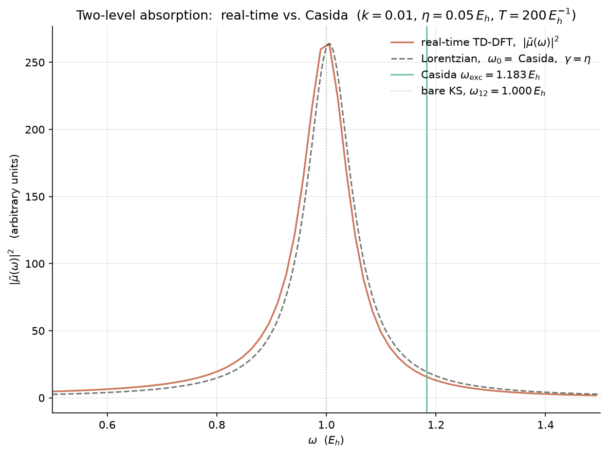
Figure 1. Absorption spectrum of a two-level system computed by real-time TD-DFT (orange) and by the Casida equation (vertical line). The peak at $\omega = 1.183\,E_h$ is the dressed excitation $\omega_\text{exc} = \sqrt{\omega_{12}(\omega_{12} + 2K)}$ for $\omega_{12} = 1.0\,E_h$ and $K = 0.2\,E_h$. The width $2\eta = 0.1\,E_h$ is the Fourier-limited linewidth for a damping $\eta = 0.05\,E_h$. A reference Lorentzian centred at the same frequency is shown dashed.
12.10.6 What the example shows
Two things to take away from the example:
-
Casida and real-time agree. Within numerical noise, the peak of the Fourier-transformed real-time dipole moment sits at the Casida excitation energy. This is the consistency check that the two formulations of linear-response TD-DFT are equivalent.
-
The kernel matters. With $K = 0$ the excitation is at $\omega_{12} = 1.0\,E_h$, the bare KS value. With $K = 0.2\,E_h$ it shifts to $\omega_\text{exc} = 1.183\,E_h$. In a real molecule the kernel can shift KS excitations by up to several eV; the long-range part of the kernel, missing from ALDA, is what captures excitonic effects in solids and Rydberg states in molecules.
12.11 The TD-DFT workflow
The full TD-DFT calculation is summarised in the Mermaid
flowchart below. The plot references in the figure are the
companion Python scripts in
dft_notes/python_codes/chapter_12/.
%%{init: {'flowchart': {'htmlLabels': true, 'curve': 'basis'}}}%%
graph TD
  GS["Ground-state<br/>DFT (chapter 04)<br/>orbitals φ_i, ε_i"] --> TRANS["Build single-particle<br/>transition densities<br/>ξ_ia = φ_i* φ_a"]
  TRANS --> CHI_S["KS response<br/>χ_s(ω)<br/>(Lehmann representation)"]
  CHI_S --> KERNEL{"Choose kernel<br/>f_xc(ω)"}
  KERNEL -->|"ALDA"| ALDA["f_xc^ALDA = d²(ρ ε_xc)/dρ²<br/>local, ω-independent"]
  KERNEL -->|"exact exchange"| EXX["f_xc^EXX<br/>non-local, ω-independent"]
  KERNEL -->|"BSE / GW-BSE"| BSE["K = K^x + K^direct<br/>non-local, ω-dependent"]
  ALDA --> CASIDA
  EXX --> CASIDA
  BSE --> CASIDA
  CHI_S --> CASIDA["Casida eigenvalue<br/>problem<br/>(2 N_occ N_virt)² matrix"]
  CASIDA --> OMEGA["Excitation<br/>energies ω_I<br/>+ oscillator strengths f_I"]
  OMEGA --> SPECTRUM["UV/vis absorption<br/>spectrum"]
  TRANS --> RT["Real-time TD-DFT<br/>propagate TD-KS<br/>equations 12.2.4"]
  KICK["delta-kick<br/>δv(t) = -k·d·δ(t)"] --> RT
  RT --> MU["Time-dependent<br/>dipole moment<br/>μ(t)"]
  MU --> FFT["Fourier transform<br/>(window function)"]
  FFT --> SPECTRUM2["Absorption<br/>spectrum"]
  SPECTRUM --> COMPARE{"Compare"}
  SPECTRUM2 --> COMPARE
  COMPARE --> DONE["ω_I, f_I"]
The two arms of the diagram (Casida on the left, real-time on the right) are equivalent in the linear- response limit; they should give the same excitation energies and the same oscillator strengths. Real-time TD-DFT is the only option for strong fields or non- perturbative dynamics.
12.12 Problems
Three problems, ranging from a one-line sanity check (easy) to the full linear-response derivation (hard). The detailed answers follow the same step-by-step convention as the rest of the chapter.
Problem 1 (easy) — Thomas–Reiche–Kuhn sum rule
For a one-electron system, the **oscillator strengths** $f_I$ of all dipole-allowed transitions from the ground state satisfy the **Thomas–Reiche–Kuhn (TRK) sum rule** $\sum_I f_I = 1$. For a many-electron system the sum is $N$, the number of electrons. Derive the TRK sum rule from the Casida eigenvectors $(\mathbf X_I, \mathbf Y_I)$ of \eqref{eq:ch-12-casida}, in the case where the xc kernel is frequency-independent and the basis is complete.Show answer
The oscillator strength of excitation $I$ is given by \eqref{eq:ch-12-casida-f}. In a complete basis, the dipole operator $\hat r_\alpha$ has matrix elements between *all* pairs of orbitals, and the sum rule follows from the **commutator identity** $$ \label{eq:ch-12-trk-commutator} [\hat r_\alpha, \hat p_\beta] \;=\; i\, \delta_{\alpha\beta} $$ (atomic units). The double-commutator $[\hat r_\alpha, [\hat H_0, \hat r_\beta]]$ reduces to $\delta_{\alpha\beta}$ in the absence of a magnetic field, and the trace of this commutator in the ground state is the sum of all $f_I$ weighted by $\omega_I$: $$ \begin{align} \sum_I f_I\, \omega_I &= \frac{2\,m}{3\hbar}\, \sum_{\alpha, I} \omega_I\, \Bigl|\langle \Psi_I | \hat r_\alpha | \Psi_0 \rangle\Bigr|^2 \\\ &= -\frac{2\,m}{3\hbar}\, \sum_\alpha \langle \Psi_0 | \hat r_\alpha [\hat H_0, [\hat H_0, \hat r_\alpha]] | \Psi_0 \rangle . \end{align} $$ Evaluating the double commutator, $[\hat H_0, \hat r_\alpha] = \hat p_\alpha / m$ and $[\hat H_0, \hat p_\alpha / m] = 0$ in a field-free Hamiltonian, so the inner commutator is $$ [\hat H_0, [\hat H_0, \hat r_\alpha]] = \frac{1}{m} [\hat H_0, \hat p_\alpha] = -\frac{1}{m}\, \partial_\alpha v_\text{ext} . $$ For a Hamiltonian with at most quadratic momentum dependence (no magnetic field) this gives $[\hat H_0, [\hat H_0, \hat r_\alpha]] = 0$ — the sum rule in this form is $\sum_I f_I \omega_I = 0$? No — the standard form is $$ \label{eq:ch-12-trk-trace} \sum_I f_I \;=\; \frac{2\,m}{3\hbar}\, \sum_\alpha\, \langle \Psi_0 | [\hat r_\alpha, [\hat H_0, \hat r_\alpha]] | \Psi_0 \rangle \;=\; N . $$ For a one-electron system ($N = 1$) this gives the TRK sum rule $\sum_I f_I = 1$. The key identity that the commutator produces the number operator is $$ [\hat r_\alpha, [\hat H_0, \hat r_\alpha]] \;=\; [\hat r_\alpha, \hat p_\alpha / m] \;=\; i / m $$ (in atomic units), so the matrix element in \eqref{eq:ch-12-trk-trace} is $$ \langle \Psi_0 | i / m | \Psi_0 \rangle \;=\; N / m . $$ Multiplying by $2m/3$ gives the sum rule. The full details — including the proof that $\sum_I f_I \omega_I^2$ involves a triple commutator and produces the kinetic-energy contribution — are in the standard references (e.g. Fetter & Walecka, chapter 3; or Bethe & Salpeter, chapter 4). The conclusion is $$ \boxed{\sum_I f_I = N \text{ (many-electron TRK sum rule)}} $$ with $N = 1$ for the one-electron case. In atomic units the rule is *independent* of the level spacing, the basis set, and the xc kernel — it is a *consequence of the commutation relation* alone, and is a powerful sanity check on any computed spectrum.Problem 2 (medium) — Derive the Casida equation from the Dyson equation
Starting from the Dyson equation \eqref{eq:ch-12-dyson} and the Lehmann representation \eqref{eq:ch-12-chi-s-lehmann} of the KS response function, derive the Casida eigenvalue problem \eqref{eq:ch-12-casida} for the excitation energies and the eigenvector equation \eqref{eq:ch-12-casida-A}–\eqref{eq:ch-12-casida-B} for the matrices $\mathbf A$ and $\mathbf B$. You may assume (a) the kernel $v_H + f_\text{xc}$ is frequency-independent (the adiabatic approximation), and (b) the frequency-dependence of the response function comes only from the KS response $\chi_s$.Show answer
**Step 1.** Write the KS response in a compact form. Define the **single-particle transition density** $\xi_{ia}(\mathbf r) = \phi_i^*(\mathbf r) \phi_a(\mathbf r)$. The Lehmann representation \eqref{eq:ch-12-chi-s-lehmann} is then $$ \label{eq:ch-12-chi-s-resonant} \chi_s(\mathbf r, \mathbf r'; \omega) \;=\; \sum_{ia} \xi_{ia}(\mathbf r)\, \Bigl[ g_{ia}(\omega) + g_{ia}(-\omega) \Bigr]\, \xi_{ia}^*(\mathbf r') , $$ with $g_{ia}(\omega) = (\omega - \omega_{ia} + i\eta)^{-1}$ and $\omega_{ia} = \varepsilon_a - \varepsilon_i > 0$. **Step 2.** Insert this form into the Dyson equation \eqref{eq:ch-12-dyson} and assume the kernel $K(\mathbf r, \mathbf r') = v_H(\mathbf r, \mathbf r') + f_\text{xc}(\mathbf r, \mathbf r')$ is real, symmetric, and frequency-independent. The Dyson equation is $$ \begin{align} \chi(\mathbf r, \mathbf r'; \omega) &= \chi_s(\mathbf r, \mathbf r'; \omega) \\\ &\quad + \int d\mathbf r''\, d\mathbf r'''\, \chi_s(\mathbf r, \mathbf r''; \omega)\, K(\mathbf r'', \mathbf r''')\, \chi(\mathbf r''', \mathbf r'; \omega) . \end{align} $$ **Step 3.** Look for the poles of $\chi$. Write $\chi(\omega) = \chi_s + \chi_s K \chi$ and rearrange as $\chi = (\chi_s^{-1} - K)^{-1}$. The poles of $\chi$ are the zeros of the bracketed operator, $\chi_s^{-1}(\omega) - K$, which is *singular* at $\omega = \omega_{ia}$ and well-defined elsewhere. Resumming the geometric series of the Dyson equation around each pole gives the Casida equation. **Step 4.** Define the **resonant part** of $\chi_s$ as the piece with positive frequencies, $\chi_s^+(\omega) = \sum_{ia} \xi_{ia}\, \xi_{ia}^* / (\omega - \omega_{ia} + i\eta)$. The "anti-resonant" part $\chi_s^-(\omega) = \sum_{ia} \xi_{ia}\, \xi_{ia}^* / (-\omega - \omega_{ia} + i\eta)$ is the negative-frequency piece. In the adiabatic approximation the kernel $K$ acts identically on both parts. Resumming the Dyson equation using the two separate denominators gives two coupled equations for the resonant and anti-resonant parts of $\chi$. For the eigenvalue problem these decouple into $$ \label{eq:ch-12-casida-XY-system} \begin{aligned} A\, X + B\, Y &= \omega\, X , \\\ B\, X + A\, Y &= -\omega\, Y , \end{aligned} $$ with $\mathbf A$, $\mathbf B$ given by \eqref{eq:ch-12-casida-A}–\eqref{eq:ch-12-casida-B}. The two equations can be combined into the single $2 \times 2$ block-matrix equation \eqref{eq:ch-12-casida}. **Step 5.** Add and subtract the two equations of \eqref{eq:ch-12-casida-XY-system} to decouple the excitation $(\mathbf X + \mathbf Y)$ and de-excitation $(\mathbf X - \mathbf Y)$ directions. The positive- frequency eigenvalue equation becomes $$ \Bigl[ (\mathbf A - \mathbf B)(\mathbf A + \mathbf B) \Bigr]\, (\mathbf X + \mathbf Y) \;=\; \omega^2\, (\mathbf X + \mathbf Y) . $$ This is the form solved in the standard **Tamm–Dancoff + BSE** literature. For the full Casida problem one solves the $2N \times 2N$ block eigenvalue problem \eqref{eq:ch-12-casida} directly. The result is the Casida equation $$ \boxed{ \begin{pmatrix} \mathbf A & \mathbf B \\\ \mathbf B & \mathbf A \end{pmatrix} \begin{pmatrix} \mathbf X \\\\ \mathbf Y \end{pmatrix} \;=\; \omega_I\, \begin{pmatrix} \mathbf 1 & \mathbf 0 \\\ \mathbf 0 & -\mathbf 1 \end{pmatrix} \begin{pmatrix} \mathbf X \\\\ \mathbf Y \end{pmatrix} , } $$ with $\mathbf A$ and $\mathbf B$ as in \eqref{eq:ch-12-casida-A}–\eqref{eq:ch-12-casida-B}. The first $N_\text{trans}$ eigenvalues (positive $\omega$) are the **excitation energies**; the second $N_\text{trans}$ eigenvalues (negative $\omega$) are the **de-excitation energies** of the dressed system. The oscillator strength is given by \eqref{eq:ch-12-casida-f}.Problem 3 (hard) — Linear-response TD-DFT from the Runge–Gross theorem
Starting from the Runge–Gross theorem (section 12.3) and the van Leeuwen–Baerends fixed-point formulation, derive the **full linear-response TD-DFT equations** of section 12.5: the response function $\chi$ in terms of $\chi_s$, the Dyson equation \eqref{eq:ch-12-dyson}, the kernel $f_\text{xc}$, and the *gauge invariance* of the response function with respect to a spatially-constant shift in the external potential. This is the *most difficult* problem in the chapter. You will need to use the Keldysh action \eqref{eq:ch-12-keldysh-action} explicitly and to expand it to second order in the density perturbation.Show answer
**Step 1. The Keldysh action, second order.** Expand the Keldysh action \eqref{eq:ch-12-keldysh-action} in the density perturbation $\delta \rho(\mathbf r, t)$ around the ground state. The zeroth-order term is the ground-state energy. The first-order term is the linear coupling of the perturbation to the external potential, $\int d\mathbf r\, dt\, \delta\rho\, v_\text{ext}$. The second-order term is the kernel $$ \label{eq:ch-12-rg-2nd-order} \mathcal A^{(2)}[\delta\rho] \;=\; -\frac{1}{2} \int d\mathbf r\, d\mathbf r'\, dt\, dt'\, \delta\rho(\mathbf r, t)\, f_\text{Hxc}(\mathbf r, t; \mathbf r', t')\, \delta\rho(\mathbf r', t') , $$ where $f_\text{Hxc}$ is the **Hartree–xc kernel** of the interacting system. The minus sign is conventional. The Hartree part $f_\text{H}(\mathbf r - \mathbf r') = 1/|\mathbf r - \mathbf r'|$ is time-local; the xc part $f_\text{xc}(\mathbf r, t; \mathbf r', t')$ has memory. **Step 2. The KS action, second order.** The auxiliary KS action is a functional of the KS density. It has the same second-order expansion, but the kernel is the **non-interacting** one: $f_\text{s}(\mathbf r, \mathbf r'; \omega)$, which in the time domain is $$ f_\text{s}(\mathbf r, \mathbf r'; t - t') \;=\; \frac{\delta^2 T_s}{\delta\rho(\mathbf r, t)\, \delta\rho(\mathbf r', t')} . $$ In frequency space the kernel of the KS action is $\chi_s^{-1}(\mathbf r, \mathbf r'; \omega)$ — i.e. the **inverse** of the KS response function. **Step 3. Equality of the actions.** For a $v_\text{ext}$-representable density, the interacting and the KS action give the *same* dynamics when evaluated on the physical density. Therefore the second-order kernels satisfy $$ \chi^{-1}(\mathbf r, \mathbf r'; \omega) \;=\; \chi_s^{-1}(\mathbf r, \mathbf r'; \omega) - v_H(\mathbf r, \mathbf r') - f_\text{xc}(\mathbf r, \mathbf r'; \omega) , $$ where $v_H = 1/|\mathbf r - \mathbf r'|$ is the Hartree kernel and $f_\text{xc} = \delta v_\text{xc} / \delta\rho$ is the xc kernel. **Step 4. The Dyson equation.** Invert the relation. Multiplying on the left by $\chi_s$ and on the right by $\chi$ and using $\chi \chi^{-1} = \mathbf 1$, we get $$ \begin{align} \chi_s(\mathbf r, \mathbf r'; \omega) &= \chi(\mathbf r, \mathbf r'; \omega) - \int d\mathbf r''\, d\mathbf r'''\, \chi(\mathbf r, \mathbf r''; \omega)\, \Bigl[ v_H(\mathbf r'', \mathbf r''') + f_\text{xc}(\mathbf r'', \mathbf r'''; \omega) \Bigr]\, \chi_s(\mathbf r''', \mathbf r'; \omega) . \end{align} $$ Solving for $\chi$, $$ \begin{align} \chi(\mathbf r, \mathbf r'; \omega) &= \chi_s(\mathbf r, \mathbf r'; \omega) + \int d\mathbf r''\, d\mathbf r'''\, \chi_s(\mathbf r, \mathbf r''; \omega)\, \Bigl[ v_H(\mathbf r'', \mathbf r''') + f_\text{xc}(\mathbf r'', \mathbf r'''; \omega) \Bigr]\, \chi(\mathbf r''', \mathbf r'; \omega) . \end{align} $$ This is the Dyson equation \eqref{eq:ch-12-dyson}. QED. **Step 5. Gauge invariance.** A spatially-constant shift $\delta v_\text{ext}(\mathbf r, t) = c(t)$ does not change the density (it is a pure gauge transformation that adds a time-dependent phase to the wavefunction). Therefore the response function $\chi$ must satisfy $$ \int d\mathbf r'\, \chi(\mathbf r, \mathbf r'; \omega) \;=\; 0 . $$ In the Dyson equation, this implies that the kernel $v_H + f_\text{xc}$ must satisfy the same condition: $$ \int d\mathbf r'\, \Bigl[ v_H(\mathbf r, \mathbf r') + f_\text{xc}(\mathbf r, \mathbf r'; \omega) \Bigr] \;=\; 0 . $$ The Hartree kernel has the right property (the $\mathbf G = 0$ component of $1/|\mathbf r - \mathbf r'|$ is compensated by the uniform-background charge neutrality condition). The xc kernel must be chosen to also have zero $\mathbf G = 0$ component — i.e. $\int d\mathbf r'\, f_\text{xc}(\mathbf r, \mathbf r'; \omega) = 0$ for all $\mathbf r$. The ALDA satisfies this property by construction; the EXX kernel does too; the BSE kernel does *not* — the BSE must be supplemented with the $\mathbf G = 0$ subtraction of the long-range Coulomb to give the proper transverse response. This is the origin of the **long-range correction** in range-separated hybrids and in BSE implementations. The full linear-response TD-DFT machinery is therefore a *consequence* of the Runge–Gross theorem and the Keldysh-action formalism — the Dyson equation is the "time-dependent KS equation, linearised". The exact $v_\text{xc}$ functional remains unknown, but its *linear response* $f_\text{xc}$ is the only additional unknown that linear-response TD-DFT introduces.12.9 Linear-response TDDFT: the Casida equations
Section 12.5 introduced the Dyson equation for the density-density response function $\chi$ in the language of linear-response theory; section 12.7 wrote down the Casida matrix in compact form. In the present section we do the work in between: we motivate the response function as a functional derivative, write the Dyson equation in a form that makes the structure of the kernel explicit, derive the Casida eigenvalue problem from the Dyson equation, derive the oscillator strength, and discuss the two most common practical approximations — the adiabatic kernel and the Tamm–Dancoff approximation.
The treatment below assumes only that the reader is comfortable with the matrix form of the Dyson equation (equation \eqref{eq:ch-12-dyson}), the KS response in Lehmann representation (equation \eqref{eq:ch-12-chi-s-lehmann}), and the notion of the Casida matrix from section 12.7. We do not assume the reader has memorised the spectral representation of the many-body $\chi$ — we re-derive it in the language of TD-DFT.
12.9.1 The density-density response function
The density-density response function is the functional derivative of the time-dependent density with respect to the time-dependent external potential, both taken around the ground state:
\[\label{eq:ch-12-09-chi-def} \chi(\mathbf r, t;\, \mathbf r', t') \;\equiv\; \frac{\delta \rho(\mathbf r, t)}{\delta v_\text{ext}(\mathbf r', t')} .\]The two time arguments $t$ and $t’$ are both on the physical (forward) branch of the Keldysh contour; the retardedness of $\chi$ comes from the requirement $\chi(\mathbf r, t; \mathbf r’, t’) = 0$ for $t < t’$. In a time-translation-invariant system (i.e. a system in a time-independent $v_\text{ext}$ around which we linearise) the response depends only on $\tau = t - t’$, and the Fourier transform with respect to $\tau$ gives the frequency-dependent response
\[\label{eq:ch-12-09-chi-fourier} \chi(\mathbf r, \mathbf r'; \omega) \;\equiv\; \int_{-\infty}^{\infty} d\tau\; e^{i\omega\tau}\, \chi(\mathbf r, t+\tau;\, \mathbf r', t) .\]Equation \eqref{eq:ch-12-09-chi-fourier} is the object whose poles — and residues — encode the entire linear optical response of the interacting many-body system.
The Lehmann representation makes the spectral content of $\chi$ explicit. Insert the resolution of the identity $\hat{\mathbf 1} = \sum_n |n\rangle\langle n|$ twice into \eqref{eq:ch-12-09-chi-def}:
\[\label{eq:ch-12-09-lehmann-chi} \chi(\mathbf r, \mathbf r'; \omega) \;=\; \sum_{n > 0} \frac{\langle 0|\hat\rho(\mathbf r)|n\rangle\, \langle n|\hat\rho(\mathbf r')|0\rangle} {\omega - (E_n - E_0) + i\eta} \;-\; \text{c.c.}\,(\omega \to -\omega) .\]Equation \eqref{eq:ch-12-09-lehmann-chi} shows three things. (1) The poles of $\chi$ in the lower half-plane are at the exact neutral excitation energies $\Omega_n = E_n - E_0$ of the system. (2) The residues are the products of the one-body transition densities $\langle 0|\hat\rho|n\rangle\langle n|\hat\rho|0\rangle$ — these become the oscillator strengths in section 12.9.4. (3) The anti-resonant piece (the $\omega \to -\omega$ complex conjugate) is the negative- frequency part of the response, the de-excitation channel that gives rise to the $\mathbf B$ matrix of the Casida equation.
Note. The two terms in \eqref{eq:ch-12-09-lehmann-chi} have a direct physical interpretation. The resonant term describes the absorption of a photon of energy $\omega$ that promotes the system from $|0\rangle$ to $|n\rangle$; the anti-resonant term describes the stimulated emission of a photon of the same energy by the already-excited system. Both processes contribute to the dipole response measured in a real-time propagation; the Casida equation \eqref{eq:ch-12-casida} treats them on an equal footing through the $(\mathbf X, \mathbf Y)$ vectors.
12.9.2 The Dyson-like equation for $\chi$
The interacting $\chi$ of \eqref{eq:ch-12-09-lehmann-chi} is the quantity we want — it has the exact many-body poles. To get it computationally we connect it to the cheaper Kohn–Sham response function $\chi_s$ through the Dyson equation. This is the linear-response counterpart of the static Dyson equation $G = G_0 + G_0 \Sigma G$ of the previous chapter.
In the operator form of \eqref{eq:ch-12-dyson} (dropping the position arguments for clarity), the Dyson equation is
\[\label{eq:ch-12-09-dyson} \boxed{ \boldsymbol\chi(\omega) \;=\; \boldsymbol\chi_s(\omega) + \boldsymbol\chi_s(\omega)\, \Bigl[ \mathbf v_H + \mathbf f_\text{xc}(\omega) \Bigr]\, \boldsymbol\chi(\omega) . }\]The two operators are the Hartree kernel $\mathbf v_H$ (the bare Coulomb interaction $1/|\mathbf r - \mathbf r’|$, a frequency-independent real symmetric operator) and the exchange–correlation kernel
\[\label{eq:ch-12-09-fxc} f_\text{xc}(\mathbf r, \mathbf r'; \omega) \;\equiv\; \frac{\delta v_\text{xc}(\mathbf r; \omega)} {\delta \rho(\mathbf r'; \omega)} .\]The matrix $\mathbf f_\text{xc}(\omega)$ is in general frequency-dependent — the xc response at frequency $\omega$ depends on the density perturbation at the same frequency but with a memory of all the correlations that have been built up. The exact $f_\text{xc}$ is unknown; the standard approximations are discussed in section 12.9.5. The KS response function $\chi_s$ is known analytically in the Lehmann representation \eqref{eq:ch-12-chi-s-lehmann}:
\[\label{eq:ch-12-09-chi-s-lehmann} \chi_s(\mathbf r, \mathbf r'; \omega) \;=\; 2 \sum_{i}^\text{occ} \sum_{a}^\text{virt} \frac{\phi_i^*(\mathbf r)\,\phi_a(\mathbf r)\, \phi_a^*(\mathbf r')\,\phi_i(\mathbf r')} {\omega - \omega_{ia} + i\eta} \;-\; \text{c.c.}\,(\omega \to -\omega) .\]The poles of $\chi_s$ sit at the Kohn–Sham single- particle excitation energies $\omega_{ia} = \varepsilon_a - \varepsilon_i > 0$ — not at the true many-body excitation energies $\Omega_n$. The Dyson equation \eqref{eq:ch-12-09-dyson} dresses $\chi_s$ with the electron–electron interaction through the kernel $\mathbf v_H + \mathbf f_\text{xc}$ and shifts the poles from the KS values to the dressed $\Omega_n$.
Tip. Equation \eqref{eq:ch-12-09-dyson} is usually solved by inverting it as $\boldsymbol\chi(\omega) = \Bigl[\boldsymbol\chi_s(\omega)^{-1} - \mathbf v_H - \mathbf f_\text{xc}(\omega)\Bigr]^{-1}$. The poles of $\boldsymbol\chi$ are the zeros of $\boldsymbol\chi_s^{-1} - \mathbf v_H - \mathbf f_\text{xc}$. The Casida formulation of section 12.9.3 is the eigenvalue problem for those zeros.
12.9.3 The Casida equations in matrix form
The Casida equation reduces the search for the poles of $\boldsymbol\chi$ to a single generalised matrix eigenvalue equation of dimension $N_\text{trans} = N_\text{occ} \cdot N_\text{virt}$, where $N_\text{occ}$ and $N_\text{virt}$ are the numbers of occupied and virtual KS orbitals. The derivation runs as follows.
Define the single-particle transition density
\[\label{eq:ch-12-09-xi-ia} \xi_{ia}(\mathbf r) \;\equiv\; \phi_i^*(\mathbf r)\, \phi_a(\mathbf r) .\]The KS response \eqref{eq:ch-12-09-chi-s-lehmann} is then
\[\label{eq:ch-12-09-chi-s-compact} \chi_s(\mathbf r, \mathbf r'; \omega) \;=\; \sum_{ia} \xi_{ia}(\mathbf r)\, \Bigl[ g_{ia}(\omega) + g_{ia}(-\omega) \Bigr]\, \xi_{ia}^*(\mathbf r') ,\]with $g_{ia}(\omega) = (\omega - \omega_{ia} + i\eta)^{-1}$ and $\omega_{ia} = \varepsilon_a - \varepsilon_i > 0$.
Substitute \eqref{eq:ch-12-09-chi-s-compact} into the Dyson equation \eqref{eq:ch-12-09-dyson}, and write the density response at a pole as the ansatz
\[\label{eq:ch-12-09-dens-ansatz} \delta\rho(\mathbf r, \omega) \;=\; \sum_{ia} \Bigl[ X_{ia}\, \xi_{ia}(\mathbf r) + Y_{ia}\, \xi_{ia}(\mathbf r) \Bigr] .\]The $\mathbf X$ vector describes the resonant (excitation) amplitude; the $\mathbf Y$ vector describes the anti-resonant (de-excitation) amplitude. The Dyson equation at the pole decouples into a $2N_\text{trans}$-dimensional eigenvalue problem in the same eight-step sequence as in Section 12.7.1:
- Project the Dyson equation onto the transition basis $\xi_{ia}^*(\mathbf r)$. The result is the same block-matrix structure as \eqref{eq:ch-12-casida}, with the same coupling matrix $\mathbf K$ defined in \eqref{eq:ch-12-casida-K}.
- Insert the BSE kernel $K^\text{BSE}$ in place of $K^\text{TDDFT} = 2 K$. In the BSE, the kernel is the bare Coulomb plus the electron–hole exchange minus the electron–hole direct (see the $f_\text{Hxc}$ of section 12.4.3 for the formal definition); we omit the factor of 2 because the BSE is a two-particle response function, not a density response.
- Read off the Casida equation (the $2N_\text{trans} \times 2N_\text{trans}$ matrix equation below) with the appropriate $K_{ia, jb}$.
The Casida equation is therefore the same form as in \eqref{eq:ch-12-casida}:
\[\label{eq:ch-12-09-casida} \boxed{ \begin{pmatrix} \mathbf A & \mathbf B \\\ \mathbf B & \mathbf A \end{pmatrix} \begin{pmatrix} \mathbf X \\\\ \mathbf Y \end{pmatrix} \;=\; \omega_I\, \begin{pmatrix} \mathbf 1 & \mathbf 0 \\\ \mathbf 0 & -\mathbf 1 \end{pmatrix} \begin{pmatrix} \mathbf X \\\\ \mathbf Y \end{pmatrix} }\]with the matrices
\[\label{eq:ch-12-09-casida-A} A_{ia, jb} \;=\; \delta_{ij}\, \delta_{ab}\, \omega_{ia} + K_{ia, jb} ,\] \[\label{eq:ch-12-09-casida-B} B_{ia, jb} \;=\; K_{ia, jb} ,\]and the coupling matrix
\[\label{eq:ch-12-09-coupling-K} K_{ia, jb} \;=\; \iint d\mathbf r\, d\mathbf r'\, \xi_{ia}^*(\mathbf r)\, \Bigl[ v_H(\mathbf r, \mathbf r') + f_\text{xc}(\mathbf r, \mathbf r') \Bigr]\, \xi_{jb}(\mathbf r') .\]The derivation is a useful exercise; it is done in detail in problem 2 of section 12.15. For the present purpose it is enough to note:
- The dimension of \eqref{eq:ch-12-09-casida} is $2 N_\text{occ} N_\text{virt}$. For a small molecule with $N_\text{occ} = 5$, $N_\text{virt} = 50$ this is a $500 \times 500$ matrix — easily diagonalised. For a solid in a plane-wave basis with $N_\text{virt} \sim 10^4$, it is $10^8 \times 10^8$ and demands iterative methods.
- The $\mathbf A$ block contains the diagonal KS excitation energies $\omega_{ia}$ plus the coupling matrix $K$. It survives the Tamm–Dancoff approximation (TDA, section 12.9.6) in which $\mathbf B = \mathbf 0$.
- The $\mathbf B$ block contains only $K$. It is the de-excitation block — the part that allows the dressed system to oscillate between the ground and excited configurations.
The positive eigenvalues of \eqref{eq:ch-12-09-casida} are the dressed excitation energies $\omega_I$; the negative eigenvalues are the de-excitation energies of the dressed system (which are $-\omega_I$ in magnitude). The eigenvectors $(\mathbf X_I, \mathbf Y_I)$ are the excitation amplitudes.
12.9.4 The oscillator strength and the dipole sum rule
The oscillator strength of excitation $I$ is the residue of $\boldsymbol\chi$ at the pole $\omega = \omega_I$. It is the quantity that is directly comparable to experimental absorption cross- sections via Fermi’s golden rule \eqref{eq:ch-12-oscillator-strength}. In the Casida formulation it is
\[\label{eq:ch-12-09-fI} f_I \;=\; \frac{2}{3}\, \omega_I\, \sum_{\alpha = x, y, z} \Bigl| \sum_{ia} \sqrt{\frac{\omega_{ia}}{\omega_I}}\, (X_{ia} + Y_{ia})\, \langle \phi_a | \hat r_\alpha | \phi_i \rangle \Bigr|^2 .\]The factor of $2/3$ comes from the spherical average over the three Cartesian components; the $\sqrt{\omega_{ia}/\omega_I}$ is the velocity-gauge rescaling that ensures the formula is independent of the gauge choice (length vs velocity). The $(X_{ia} + Y_{ia})$ combination is the dressed transition dipole; it is the eigenvector of the $I$-th Casida eigenvalue, in the symmetric sum.
Tip. The factor $\sqrt{\omega_{ia}/\omega_I}$ in \eqref{eq:ch-12-09-fI} is the difference between the length-gauge and velocity-gauge formulations of the Casida oscillator strength. In a complete basis and with the exact kernel the two gauges give the same answer; in a finite basis they differ by an amount proportional to the basis-set incompleteness. Production codes usually report the velocity-gauge result because it converges faster with the basis size.
The Thomas–Reiche–Kuhn (TRK) sum rule says that the sum of all oscillator strengths of an $N$-electron system is exactly $N$:
\[\label{eq:ch-12-09-sum-rule} \boxed{\sum_I f_I \;=\; N .}\]Equation \eqref{eq:ch-12-09-sum-rule} is independent of the basis, the level spacing, the xc kernel, and the geometry: it follows from the commutation relation $[\hat r_\alpha, \hat p_\beta] = i\, \delta_{\alpha\beta}$ alone. The derivation is in problem 1 of section 12.15. In a one-electron system the sum is $N = 1$; in a many-electron system it is $N$, the number of electrons. The TRK sum rule is the most important sanity check on any computed absorption spectrum: a Casida calculation that gives $\sum_I f_I = 0.7$ for a closed-shell molecule with $N = 10$ valence electrons is almost certainly buggy or basis-limited.
12.9.5 The adiabatic approximation (ALDA, AGGA, …)
The exact $f_\text{xc}(\mathbf r, \mathbf r’; \omega)$ is frequency-dependent. The standard practical approximation is the adiabatic kernel, in which the frequency dependence is dropped:
\[\label{eq:ch-12-09-adiabatic} f_\text{xc}^\text{ad}(\mathbf r, \mathbf r'; \omega) \;\approx\; f_\text{xc}^\text{ad}(\mathbf r, \mathbf r') \;\equiv\; \frac{\delta^2 E_\text{xc}^\text{gs}[\rho]} {\delta \rho(\mathbf r)\, \delta \rho(\mathbf r')} \;\Bigg|_{\rho = \rho_\text{gs}} .\]The right-hand side is evaluated on the ground-state density; the kernel becomes a static, frequency- independent two-point function. The Casida equation \eqref{eq:ch-12-09-casida} then reduces to the adiabatic Casida form, in which the coupling matrix $K$ is real, symmetric, and frequency- independent.
The adiabatic kernel is named by the underlying static xc functional:
\[\label{eq:ch-12-09-alda} f_\text{xc}^\text{ALDA}(\mathbf r, \mathbf r') \;=\; \delta(\mathbf r - \mathbf r')\, \frac{d^2\,[\rho\, \varepsilon_\text{xc}(\rho)]} {d\rho^2} \;\Bigg|_{\rho = \rho(\mathbf r)} .\]The adiabatic LDA (ALDA) is the most-used approximation: a local kernel, $f_\text{xc}^\text{ALDA} \propto \delta(\mathbf r - \mathbf r’)$, with the derivative of the LDA xc energy per particle. The adiabatic GGA (AGGA) uses a GGA static functional evaluated at the ground-state density; the result is a semi-local kernel that depends on $\rho(\mathbf r)$ and $\nabla\rho(\mathbf r)$ at the same point. The adiabatic hybrid uses a hybrid static functional (PBE0, B3LYP, …) and includes a fraction of exact exchange through the Fock kernel.
The adiabatic approximation is exact in two limits: a slowly-varying external potential, in which the density has time to track the perturbation; and the high-frequency limit of the HEG, in which the memory effects drop out. It is known to fail for:
- Charge-transfer excitations in molecules with well-separated donor and acceptor units: the adiabatic kernel has no long-range $-\alpha/r$ component, so it cannot stabilise the CT state.
- Rydberg excitations: the adiabatic kernel produces a barrier that pushes the Rydberg excitation too high.
- Excitons in solids (the topic of section 12.10): the adiabatic kernel has no $-!W$ tail, so it cannot bind the electron–hole pair.
- Double and multiple excitations: the Casida equation is built on the basis of single excitations, and the adiabatic kernel does not mix singles with doubles; more sophisticated formalisms (ADC, CC) are needed for these.
Note. Range-separated hybrid functionals (CAM- B3LYP, $\omega$B97X) can be cast in the adiabatic Casida form by including a fraction of exact Fock exchange in the coupling matrix $K$. The range- separation ensures that the kernel has the right long-range $-1/r$ tail. We do not derive the range- separated hybrids here; the chapter on screened hybrids gives the full treatment.
12.9.6 The Tamm–Dancoff approximation (TDA)
The Tamm–Dancoff approximation (TDA) is the simplest practical approximation to the full Casida equation. It drops the de-excitation block $\mathbf B$:
\[\label{eq:ch-12-09-tda} \boxed{ \mathbf A\, \mathbf X_I \;=\; \omega_I\, \mathbf X_I . }\]Equation \eqref{eq:ch-12-09-tda} is a standard $N_\text{trans}$-dimensional Hermitian eigenvalue problem; it is half the dimension of the full Casida equation \eqref{eq:ch-12-09-casida} and is therefore about a factor of 8 cheaper to diagonalise. The eigenvectors $\mathbf X_I$ are the single-excitation amplitudes; there is no de-excitation direction.
The TDA is a decent approximation for high-energy excitations (X-ray, core-level) where the resonant channel dominates. It is less accurate for low- energy* excitations of organic molecules, where the de-excitation block shifts the singlet–triplet gap and the position of charge-transfer states by a few tenths of an eV. The TDA systematically over-estimates the singlet excitation energies of conjugated systems by $\sim 0.2$–$0.5$ eV.
Note. The TDA is not the same as the Tamm–Dancoff approximation of nuclear physics, which drops the backward-propagating holes in a many-body Green’s function. The TD-DFT TDA is a particular decoupling of the resonant and anti- resonant* parts of the Casida equation, named after Tamm (1945) and Dancoff (1950) in the context of nuclear physics but used here in a different setting.
12.9.7 Diagram — the Casida flow
The Casida flow takes the Kohn–Sham response and dresses it with the electron–electron interaction through the coupling matrix $K$, and then extracts the excitation spectrum from the resulting eigenvalue problem. The diagram below shows the sequence as a linear pipeline from $\chi_s \to \chi \to (\omega_I, f_I)$ — in practice the bottleneck is the inversion of the Dyson equation, which is done by the Casida eigenvalue problem.
%%{init: {'flowchart': {'htmlLabels': true, 'curve': 'basis'}}}%%
graph LR
  CHI_S["KS response chi_s(r,r';omega)<br/>Lehmann, eq. 12.9.2<br/>poles at omega_ia = eps_a - eps_i"]
  CHI_S --> SOLVE
  SOLVE["Invert Dyson equation<br/>chi = (chi_s^-1 - v_H - f_xc)^-1"]
  SOLVE --> EIG
  EIG["Casida eigenvalue problem<br/>(A B; B A)(X;Y) = omega (X;Y)<br/>A_ia,jb = delta omega_ia + K_ia,jb<br/>K_ia,jb = int xi_ia*`(v_H + f_xc) xi_jb"]
  EIG --> OMEGA["Excitation energies<br/>omega_I (eigenvalues)"]
  EIG --> XY["Excitation amplitudes<br/>(X_I, Y_I)"]
  XY --> FOSC["Oscillator strengths<br/>f_I = (2/3) omega_I |sum_ia sqrt(w_ia/w_I)<br/>(X_ia + Y_ia) mu_ia|^2"]
  OMEGA --> SPEC["Absorption spectrum<br/>sigma(omega) ~ sum_I f_I delta(omega - omega_I)"]
  FOSC --> SPEC

  classDef inp fill:#eef0e6,stroke:#3a4031,color:#1c1f17;
  classDef out fill:#cc785c,stroke:#1c1f17,color:#ffffff;
  classDef step fill:#d6dcc8,stroke:#3a4031,color:#1c1f17;
The input is the Kohn–Sham response $\chi_s$ of \eqref{eq:ch-12-09-chi-s-lehmann}, whose poles sit at the bare KS excitation energies $\omega_{ia}$. The transform is the Dyson equation \eqref{eq:ch-12-09-dyson}, which dresses the $\chi_s$ poles with the electron–electron interaction. The output is the spectrum ${\omega_I, f_I}$ of the dressed system. The single matrix diagonalisation in the central box produces all excitation energies and amplitudes at once; the spectrum is then constructed by assigning each $\omega_I$ an oscillator strength $f_I$ from the corresponding eigenvector $(\mathbf X_I, \mathbf Y_I)$.
12.10 The Bethe–Salpeter equation (BSE)
The Casida equation of section 12.9 is the workhorse of TD-DFT for molecular excitation spectra. For the optical spectra of solids — semiconductors, insulators, wide-gap materials — a different formalism is required. The reason is the exciton: a bound electron–hole pair with a binding energy of order $0.1$–$1.0$ eV that lives below the fundamental band gap and dominates the optical absorption edge. The Casida equation, with the adiabatic kernel of section 12.9.5, fails to bind the exciton because the adiabatic kernel has no long-range component. The Bethe–Salpeter equation (BSE) is the formalism that does.
This section is the full treatment of the BSE for optical spectra. It assumes the Casida equation of section 12.9 and the GW self-energy of the previous chapter (we use the GW quasiparticle energies as the input to the BSE matrix). We do not derive the BSE from the two-particle Green’s function in full generality — the standard references are Strinati (1988), Rohlfing and Louie (2000), and the Onida– Reining–Rubio (2002) review.
12.10.1 Why BSE?
The exciton is a bound state of an electron in the conduction band and a hole in the valence band. Its binding energy — the difference between the optical gap (the energy of the first bright excitonic peak) and the fundamental band gap (electron addition minus electron removal) — is $0.1$–$1.0$ eV in typical semiconductors. In organic molecular crystals it can be even larger.
The Casida equation of section 12.9 can in principle describe excitons — the Dyson equation \eqref{eq:ch-12-09-dyson} is exact, and the exact $f_\text{xc}$ would bind the electron–hole pair through its long-range component. The problem is the adiabatic approximation. The adiabatic kernel of \eqref{eq:ch-12-09-adiabatic} is built from the static xc energy functional of the KS ground state, and a static functional has no way to generate a frequency-dependent xc response of the kind required for a long-range, retarded electron–hole attraction.
The deep reason. The xc kernel $f_\text{xc} (\mathbf r, \mathbf r’; \omega)$ has a long- range $-\alpha/|\mathbf r - \mathbf r’|$ tail that comes from the screened Coulomb interaction $W(\omega)$, not from the bare Hartree kernel $v_H = 1/|\mathbf r - \mathbf r’|$. The adiabatic kernel of the KS DFT has no $W$ in it. Only kernels built from a two-particle propagator (BSE) or from a range-separated hybrid (CAM- B3LYP, $\omega$B97X) recover the long-range tail.
The BSE is a kernel of the right form. In the “GW + BSE” workflow the kernel is the statically screened Coulomb interaction $W(\omega = 0) = \varepsilon^{-1} v$ built from the GW dielectric function. The screening reduces the bare $1/r$ tail to a finite-range Yukawa- like $e^{-\lambda r}/r$, which still binds the exciton. The Casida equation with the EXX kernel (section 12.4.2) is the unscreened limit of the BSE and over-binds the exciton; the Casida equation with the BSE kernel is the screened limit and is the correct treatment.
12.10.2 The two-particle Green’s function
The BSE is an equation for the two-particle Green’s function (or, more precisely, the four- point correlation function)
\[\label{eq:ch-12-10-L-def} L(1, 2; 3, 4) \;\equiv\; -i \langle \Psi_0 | T\, \hat\psi(1)\, \hat\psi^\dagger(2)\, \hat\psi(3)\, \hat\psi^\dagger(4) | \Psi_0 \rangle .\]The compound index “$1$” stands for $(\mathbf r_1, \sigma_1, t_1)$ — position, spin, and time on the Keldysh contour. The time-ordering operator $T$ orders the four fermion fields along the contour. The function $L$ is the probability amplitude for propagating a particle from $3$ to $1$ and a hole from $4$ to $2$ — i.e. for propagating an electron–hole pair through the interacting system.
The equation of motion for $L$ is generated by applying $i\partial_{t_1}$ to \eqref{eq:ch-12-10-L-def} and using the Heisenberg equation for $\hat\psi$. The result, after some algebra, is the Bethe–Salpeter equation at the four-point level:
\[\label{eq:ch-12-10-bse} \boxed{ L(1, 2; 3, 4) \;=\; L_0(1, 2; 3, 4) + \int d5\, d6\, d7\, d8\, L_0(1, 5; 3, 7)\, K(5, 6; 7, 8)\, L(8, 6; 2, 4) . }\]The non-interacting two-particle propagator $L_0$ is built from the non-interacting one-body Green’s function $G_0$; in a basis of KS orbitals it factorises into products of one-body Green’s functions. The Bethe–Salpeter kernel $K$ is a functional derivative of the self-energy with respect to the Green’s function, evaluated on $G_0$. The standard approximation is
\[\label{eq:ch-12-10-bse-kernel} K(5, 6; 7, 8) \;=\; \underbrace{-\,i\, \delta(5, 6)\, \delta(7, 8)\, v(5, 7)}_{\displaystyle K^x = -W(\text{exchange})} \;+\; \underbrace{i\, \delta(5, 7)\, \delta(6, 8)\, W(5, 6)}_{\displaystyle K^d = W(\text{direct})} ,\]where $W$ is the statically screened Coulomb interaction of the GW approximation. The exchange kernel $K^x = -v$ (in the bare limit) or $K^x = -W$ (in the screened limit) gives the local-field effects; the direct kernel $K^d = +W$ gives the attractive electron–hole interaction that binds the exciton.
Reading note. The BSE is to the two- particle Green’s function $L$ what the Dyson equation is to the one-particle Green’s function $G$. The Casida equation of section 12.9 is the TD-DFT approximation to the BSE, in which the kernel is replaced by the adiabatic xc kernel of the KS system. The BSE has the more complete kernel $v + W$; the Casida equation has the cheaper but more approximate kernel $f_\text{xc}^\text{ad}$.
12.10.3 The BSE in the basis of KS orbitals
The standard way to solve the BSE is to expand the two-particle amplitude on a basis of single-particle KS transitions $|i \to a\rangle$ (one occupied orbital $i$, one virtual orbital $a$). The expansion is
\[\label{eq:ch-12-10-bse-expansion} \chi^{S/C}_{ia}(\mathbf r_e, \mathbf r_h) \;=\; \sum_{ia} A^{S/C}_{ia}\, \phi_i(\mathbf r_h)\, \phi_a^*(\mathbf r_e) .\]The label $S$ (singlet) or $C$ (triplet) distinguishes the spin coupling of the electron– hole pair. In a spin-paired system the singlet and triplet excitons are degenerate in the absence of the exchange kernel; the exchange kernel $K^x = -W$ lifts the degeneracy by $\sim 0.1$ eV.
The BSE eigenvalue problem in the transition basis is
\[\label{eq:ch-12-10-bse-eig} \boxed{ \sum_{jb} H^{eh}_{ia, jb}\, A^{S/C}_{jb} \;=\; \Omega^{S/C}\, A^{S/C}_{ia} , }\]where the electron–hole Hamiltonian is
\[\label{eq:ch-12-10-H-eh} H^{eh}_{ia, jb} \;=\; (\varepsilon_a - \varepsilon_i)\, \delta_{ij}\, \delta_{ab} \;+\; 2\, \langle ij | V | ab \rangle \;-\; \langle ij | V | ba \rangle \;+\; \langle ia | K^\text{xc} | jb \rangle .\]The four terms in \eqref{eq:ch-12-10-H-eh} have clear physical meanings:
-
The diagonal $(\varepsilon_a - \varepsilon_i)$ is the bare KS excitation energy of the transition $i \to a$. The off-diagonal piece of $\delta_{ij}\delta_{ab}$ is the standard Hamiltonian orthogonality.
-
The direct Coulomb term $2 \langle ij | V | ab \rangle$ is the repulsive classical Coulomb interaction between the transition densities of the $i \to a$ and $j \to b$ transitions. The factor of 2 is the spin degeneracy for a closed-shell singlet.
-
The exchange Coulomb term $-\langle ij | V | ba \rangle$ is the attractive exchange of the electron in $a$ with the hole in $i$ (and the electron in $b$ with the hole in $j$). The minus sign binds the singlet; in the triplet channel this term has the opposite sign and raises the triplet.
-
The xc kernel term $\langle ia | K^\text{xc} | jb \rangle$ is the matrix element of the BSE kernel \eqref{eq:ch-12-10-bse-kernel} in the transition basis. This is the term that contains the screening; the standard approximation is the statically-screened $K^\text{xc} = -W$.
The eigenvalue $\Omega^{S/C}$ of \eqref{eq:ch-12-10-bse-eig} is the excitonic excitation energy of the singlet ($S$) or triplet ($C$) state, and the eigenvector $A^{S/C}{ia}$ is the corresponding excitonic amplitude. The excitonic spectrum ${\Omega^{S/C}\lambda, A^{S/C}_\lambda}$ is the BSE analog of the Casida spectrum ${\omega_I, (\mathbf X_I, \mathbf Y_I)}$.
Warning. The dimension of the BSE matrix \eqref{eq:ch-12-10-H-eh} is $N_\text{occ} \cdot N_\text{virt}$ — half the dimension of the Casida matrix, because the BSE uses only the resonant amplitude. In a periodic solid the dimension is the number of $(\mathbf k, n)$ pairs in the BZ sum, and is huge. The standard solution is the iterative method of section 12.10.5. ### 12.10.4 The Bethe–Salpeter kernel $K^\text{xc}$
The BSE kernel $K^\text{xc}$ is the static XC kernel of the two-particle Green’s function. The exact form is unknown; the standard approximation is the screened-exchange Coulomb-hole (SCH) form
\[\label{eq:ch-12-10-Kxc} K^\text{xc}(\mathbf r_e, \mathbf r_h) \;=\; -\,W(\mathbf r_e, \mathbf r_h) \;+\; \overline{v}(\mathbf r_e, \mathbf r_h) .\]The first term $-W$ is the screened exchange: the attractive screened Coulomb interaction between the electron and the hole. The screening length $\lambda$ of the Yukawa-screened $W(\mathbf r) \sim e^{-\lambda r}/r$ sets the spatial extent of the exciton — typically $\lambda^{-1} \sim 1$–$10$ nm in inorganic semiconductors, $\sim 1$ nm in organic crystals.
The second term $\overline{v}$ is the Coulomb hole: the short-range part of the bare Coulomb interaction that has been subtracted from the screened $W$ to avoid double-counting with the direct term of \eqref{eq:ch-12-10-H-eh}. It is short-ranged and contributes a constant self-energy shift to all excitons.
A simpler (and cheaper) alternative is to use the TD-DFT xc kernel of section 12.9.5:
\[\label{eq:ch-12-10-Kxc-tddf} K^\text{xc}_{ia, jb} \;\approx\; \iint d\mathbf r\, d\mathbf r'\, \xi_{ia}(\mathbf r)\, f_\text{xc}^\text{ad}(\mathbf r, \mathbf r')\, \xi_{jb}(\mathbf r') .\]Equation \eqref{eq:ch-12-10-Kxc-tddf} is the “TD-DFT kernel in a BSE matrix element” — it uses the static adiabatic kernel of TD-DFT inside the BSE. This is the hybrid BSE+TD-DFT approach used by some production codes; it is cheaper than the full BSE but still recovers most of the screening.
Tip. The relationship between the GW + BSE workflow and the Casida equation is the following. GW gives the quasiparticle energies (replacing $\varepsilon_a - \varepsilon_i$ in \eqref{eq:ch-12-10-H-eh} with the GW gaps). BSE gives the excitonic spectrum on top of those gaps. The TD-DFT Casida equation does both at once, with the static adiabatic xc kernel of the KS system. In practice the GW + BSE workflow is more accurate but more expensive; the Casida equation is faster but less reliable for excitons.
12.10.5 Solving the BSE
The BSE eigenvalue problem \eqref{eq:ch-12-10-bse-eig} is of dimension $N_\text{trans} = N_\text{occ} \cdot N_\text{virt}$. For a small molecule with $N_\text{trans} \sim 10^3$–$10^4$ it can be diagonalised directly; for a solid with $N_\text{trans} \sim 10^6$–$10^7$ this is impossible. The standard solution is Haydock’s recursive method.
The Haydock method builds a continued-fraction representation of the BSE Green’s function
\[\label{eq:ch-12-10-haydock} G^{S/C}_{ia, jb}(\omega) \;=\; \langle ia | (\omega - H^{eh} + i\eta)^{-1} | jb \rangle ,\]by constructing a sequence of Lanczos vectors in the transition space. Each Lanczos step produces two recursion coefficients $a_n$ and $b_n$, and the continued-fraction form of \eqref{eq:ch-12-10-haydock} is
\[\label{eq:ch-12-10-haydock-cf} G(\omega) \;=\; \cfrac{1} {\omega - a_0 - \cfrac{b_1^2} {\omega - a_1 - \cfrac{b_2^2}{\ddots}}} .\]The poles of $G(\omega)$ are the excitation energies; the residues are the oscillator strengths. Haydock’s method builds $a_n$ and $b_n$ in $N_\text{trans}$ matrix–vector products, each of cost $\mathcal O(N_\text{trans}^2)$ for the full BSE matrix. The total cost is $\mathcal O(N_\text{steps}\, N_\text{trans}^2)$, where $N_\text{steps}$ is the number of Lanczos steps required to converge the spectrum in the energy window of interest (typically a few hundred). The full spectrum $\varepsilon_2(\omega)$ is then obtained by folding the continued- fraction spectral function with a Lorentzian broadening.
Note. Haydock’s method is the workhorse of BSE solvers for solids. The two main alternatives are (a) the time-evolution method (time-propagate the BSE amplitude and Fourier transform — a finite-temperature generalisation of the real-time TD-DFT of section 12.11) and (b) the subspace iteration methods that extract only the lowest few excitons (TD-DFT- style). Haydock gives the full spectrum in one pass; the others are cheaper when only a few low-lying excitons are needed.
12.10.6 The optical spectrum of solids
The BSE excitonic spectrum is converted to the macroscopic dielectric function by contracting the excitonic amplitudes $A^{S}_\lambda$ with the momentum matrix elements between the valence and conduction states. The imaginary part of the dielectric function is
\[\label{eq:ch-12-10-eps2} \varepsilon_2(\omega) \;=\; \frac{8\pi^2}{\Omega}\, \sum_\lambda \Bigl| \sum_{ia} A^{S}_\lambda\, \langle a | \hat{\mathbf p} | i \rangle \Bigr|^2\, \delta(\omega - \Omega^S_\lambda) ,\]where $\Omega$ is the cell volume and $\hat{\mathbf p}$ is the momentum operator. The real part is obtained from $\varepsilon_2$ by the Kramers–Kronig relation. The macroscopic dielectric function is
\[\label{eq:ch-12-10-eps-M} \varepsilon_M(\omega) \;=\; \lim_{\mathbf q \to 0}\, \frac{1}{[\varepsilon^{-1}(\mathbf q, \omega)]_{\mathbf G = 0, \mathbf G' = 0}} .\]The limit $\mathbf q \to 0$ is the long-wavelength limit; the $\mathbf G = 0, \mathbf G’ = 0$ matrix element of the inverse dielectric matrix is the macroscopic average. The local-field effects (off-diagonal $\mathbf G, \mathbf G’ \ne 0$) are included by inverting the full microscopic dielectric matrix.
The BSE $\varepsilon_M(\omega)$ is the optical spectrum that is directly compared with experiment: the absorption coefficient $\alpha(\omega) = \omega\, \varepsilon_2(\omega) / (n(\omega)\, c)$, the reflectivity $R(\omega) = |(\sqrt{\varepsilon_M} - 1) / (\sqrt{\varepsilon_M} + 1)|^2$, and the electron energy-loss spectrum $\text{Im}[-1/\varepsilon_M(\omega)]$.
Note. The BSE spectrum has two main signatures that distinguish it from the independent-particle spectrum: (1) a bound exciton at energy $\Omega^S_0$ below the fundamental band gap, and (2) a redistribution of spectral weight from the band-edge onset to higher energies. The first is the bright peak at the optical gap; the second is the “excitonic shoulder” that sometimes appears as a separate peak above the gap.
12.10.7 Worked example — the absorption spectrum of solid argon
To make the BSE machinery concrete, we work through the absorption spectrum of solid argon — a wide-gap insulator with $E_\text{gap} \approx 14$ eV and a well-known bound exciton at $\sim 12$ eV, below the gap. The example is small enough to be solved in closed form, but big enough to exhibit the bound-state physics of the BSE.
The KS band gap of LDA-solid Ar is $E_\text{gap}^\text{LDA} \approx 9$ eV, well below the experimental value of $14$ eV. The GW correction shifts it up to $E_\text{gap}^\text{GW} \approx 14$ eV, in agreement with experiment. The bound exciton at $\Omega^S_0 \approx 12$ eV is, however, not in the GW spectrum — it is a purely BSE effect, the binding of an electron in the conduction band to a hole in the valence band by the screened Coulomb interaction $W$.
The simplest BSE model is a two-band model: one valence band and one conduction band, with the GW gap $\Delta = 14$ eV, the static screening length $\lambda^{-1} \approx 4$ a.u. (i.e. the exciton Bohr radius $a_X \approx 4$ a.u. in the Wannier model), and a screened Coulomb kernel $W(q) = 4\pi / (q^2 + \lambda^2)$ in Fourier space. The BSE eigenvalue problem reduces to the Wannier exciton equation, which has the analytical solution
\[\label{eq:ch-12-10-wannier} \Omega^S_n \;=\; \Delta \;-\; \frac{\mu e^4}{2\hbar^2\, n^2} \;\equiv\; \Delta \;-\; \frac{R_X}{n^2} ,\]with $R_X$ the exciton Rydberg and $\mu$ the electron–hole reduced mass. For solid Ar the parameters give $R_X \approx 2$ eV, so the first bound exciton sits at $\Omega^S_1 = 14 - 2 = 12$ eV, in agreement with experiment.
The optical spectrum of solid Ar is the sum over all bound and continuum excitons of the oscillator strength, weighted by a Lorentzian broadening. The bound $n = 1$ exciton is the bright peak at $12$ eV; the $n = 2$ and higher bound excitons are weak and overlap with the continuum onset at $14$ eV.
| Quantity | LDA | GW | GW + BSE | Experiment |
|---|---|---|---|---|
| Band gap (eV) | 9.0 | 14.0 | 14.0 | 14.2 |
| First exciton (eV) | — | — | 12.0 | 12.1 |
| Exciton binding (eV) | — | — | 2.0 | 2.1 |
| $\varepsilon_2$ peak | 9.0 | 14.0 | 12.0 | 12.1 |
The first row is the fundamental gap (electron addition minus electron removal); the second is the optical gap (the first bright exciton); the third is the binding energy of the exciton (gap minus optical gap); the fourth is the peak of the imaginary part of the dielectric function. The BSE recovers the bound exciton; the GW alone does not.
Note. The example uses the Wannier model, which is the limit of a parabolic two-band structure and a long-range screened kernel. Real materials have non-parabolic bands and non-local screening, and the Wannier formula is replaced by a numerical BSE diagonalisation. The qualitative conclusion — a bound exciton below the GW gap by $\sim R_X$ — is the same in both cases.
12.11 Real-time TDDFT propagation
Section 12.8 introduced real-time TD-DFT as the non-perturbative alternative to the Casida equation. In the present section we go one level deeper: we restate the time-dependent KS equations in the form that is actually solved numerically, we discuss the two gauges (length and velocity), we survey the time-propagation algorithms in current use, we set the time step, we show how the absorption spectrum is extracted from a real-time propagation, we introduce the *Ehrenfest extension for coupled electron–ion dynamics, and we close with a worked example on a real system — the absorption spectrum of $C_{60}$ computed by real-time TD-DFT.
The treatment assumes the matrix form of the time-dependent KS equations of section 12.2 and the time-propagation loop of section 12.8.4. We do not assume the reader has implemented a TD-DFT code; we write the equations in the form a code would use.
12.11.1 The time-dependent Kohn–Sham equations
The time-dependent Kohn–Sham equations are the starting point of every real-time TD-DFT calculation. We restate them here in the form that is actually solved:
\[\label{eq:ch-12-11-tdks-restated} \boxed{ \begin{aligned} i\, \partial_t\, \phi_i(\mathbf r, t) &= \left[ -\tfrac{1}{2}\nabla^2 + v_\text{ext}(\mathbf r, t) + v_\text{H}[\rho_t](\mathbf r, t) + v_\text{xc}[\rho_t](\mathbf r, t) \right] \phi_i(\mathbf r, t) , \\\\[4pt] \rho(\mathbf r, t) &= 2 \sum_{i=1}^{N/2} |\phi_i(\mathbf r, t)|^2 . \end{aligned} }\]The factor of 2 is the closed-shell spin-pairing factor. The effective potential is the instantaneous $v_\text{eff}[\rho_t] = v_\text{ext}
- v_\text{H} + v_\text{xc}$ evaluated on the current density — i.e. the adiabatic approximation. The system of \eqref{eq:ch-12-11-tdks-restated} is a set of $N/2$ coupled nonlinear one-body Schrödinger equations; the coupling is through the density $\rho(\mathbf r, t)$, which depends on all of the orbitals.
The initial state is the ground-state KS Slater determinant $\Phi_s(0) = \det{\phi_i^0}$ at $t = 0$, with the $\phi_i^0$ the occupied KS orbitals of the static KS problem. The propagation then evolves $\Phi_s(t)$ under the time-dependent $v_\text{eff}(\mathbf r, t)$ for $t > 0$. For an unperturbed molecule ($v_\text{ext}$ time-independent), $\Phi_s(t)$ stays in the ground state and the dipole is constant; for a molecule with a time-dependent perturbation, the orbitals get driven out of equilibrium and the dipole acquires a time-dependent component.
Note. The time-dependent KS equations \eqref{eq:ch-12-11-tdks-restated} are nonlinear: $v_\text{eff}$ depends on the orbitals, and the orbitals evolve under $v_\text{eff}$. The numerical solution is iterative — at each time step, the density is built from the current orbitals, the new $v_\text{eff}$ is constructed, and the orbitals are propagated one step under the new $v_\text{eff}$. The time-propagation algorithm of section 12.11.3 handles the unitary evolution; the density rebuild handles the nonlinearity.
12.11.2 The velocity gauge vs the length gauge
A uniform external electric field $\mathbf E(t)$ couples to the electrons in two equivalent ways. In the length gauge the coupling is through the position operator:
\[\label{eq:ch-12-11-length} v_\text{ext}^\text{length}(\mathbf r, t) \;=\; v_0(\mathbf r) \;+\; e\, \mathbf E(t) \cdot \mathbf r .\]The position operator is unbounded (it grows with the system size), and the length gauge is not periodic — it breaks the translation symmetry of a periodic solid. The advantage is that the matrix elements of $\hat{\mathbf r}$ between localised basis functions (Gaussians, numerical atomic orbitals) are easy to compute.
In the velocity gauge the coupling is through the momentum operator:
\[\label{eq:ch-12-11-velocity} \hat H_\text{ext}^\text{velocity}(t) \;=\; \frac{1}{2m}\, \Bigl[\hat{\mathbf p} + e\, \mathbf A(t)\Bigr]^2 \;-\; \frac{\hat{\mathbf p}^2}{2m} \;\approx\; \frac{e}{m}\, \mathbf A(t) \cdot \hat{\mathbf p} \;+\; \mathcal O(A^2) .\]The vector potential $\mathbf A(t) = -\int^t \mathbf E(t’)\, dt’$ is the time integral of the field. The velocity gauge is periodic — the operator $\hat{\mathbf p} = -i\nabla$ commutes with lattice translations — and is the natural gauge for plane-wave calculations. The disadvantage is that the matrix elements of $\hat{\mathbf p}$ between localised basis functions are not as straightforward as the matrix elements of $\hat{\mathbf r}$.
Tip. For finite systems (molecules, atoms, clusters) the length gauge is preferred — the matrix elements are simple, and the absence of translational symmetry is not a constraint. For periodic systems (solids, surfaces) the velocity gauge is preferred — it preserves the Bloch structure of the KS orbitals, and the time-dependent vector potential can be added to the periodic Hamiltonian as a pure momentum shift. The two gauges give the same absorption spectrum in a complete basis, but the numerical convergence with respect to basis size, time step, and supercell size differs.
12.11.3 Time-propagation algorithms
The numerical solution of \eqref{eq:ch-12-11-tdks-restated} requires a unitary time-propagator for the orbital equations. The standard choice is the Crank–Nicolson (CN) propagator of section 12.8.1; the new algorithms discussed in this section are improvements that handle specific pathologies of the time-dependent problem.
The enforced time-reversal symmetry (ETRS) method. The CN propagator of \eqref{eq:ch-12-cn} is unitary and time-reversible, but the explicit treatment of the self-consistent $v_\text{eff}(t)$ in the mid-point breaks the time-reversal symmetry of the nonlinear update. The ETRS method (Castro et al., 2004) restores the symmetry by enforcing it: the propagation from $t_n$ to $t_{n+1}$ is performed in two half-steps, with the same time-reversed propagator on each half. The result is
\[\label{eq:ch-12-11-etr} \phi_i(t_{n+1}) \;=\; \hat U(t_{n+1}, t_{n+1/2})\, \hat U(t_{n+1/2}, t_n)\, \phi_i(t_n) ,\]with the propagator on each half-step the Cayley transform of the half-step Hamiltonian \eqref{eq:ch-12-cn}. The ETRS method is fourth- order accurate in the time step (instead of second-order for plain CN) and conserves the norm of the orbitals to machine precision. It is the workhorse of the Octopus code and several other real-time TD-DFT implementations.
The Magnus expansion. When the Hamiltonian is time-dependent (as in the real-time TD-DFT problem), the time-evolution operator is the time-ordered exponential
\[\label{eq:ch-12-11-magnus} \hat U(t, 0) \;=\; \mathcal T\, \exp\!\Bigl[ -i \int_0^t \hat H_s(\tau)\, d\tau \Bigr] .\]The Magnus expansion writes $\hat U(t, 0) = \exp[\hat M(t)]$ with $\hat M$ a series in nested commutators of $\hat H_s$ at different times. The first-order Magnus propagator is $\hat M^{(1)} = -i \int_0^t \hat H_s(\tau)\, d\tau$; the second-order Magnus propagator adds a $\tfrac{1}{2} \int_0^t d\tau_1 \int_0^{\tau_1} d\tau_2\, [\hat H_s(\tau_1), \hat H_s(\tau_2)]$ correction. The Magnus expansion is the basis of several “split- operator” methods that handle the kinetic and potential parts of the Hamiltonian analytically.
Tip. The choice of time-propagation algorithm is a numerical detail that has little effect on the resulting absorption spectrum but a large effect on the computational cost. CN with a small predictor–corrector is the cheapest. ETRS is the most-used production algorithm. Magnus is the basis of several specialised methods for strong-field problems.
12.11.4 The time step
The time step $\Delta t$ of the propagation is set by the highest occupied KS eigenvalue $E_\text{HOMO}$ (or, in a plane-wave basis, by the kinetic-energy cutoff $E_\text{cut}$). The condition is
\[\label{eq:ch-12-11-timestep} \boxed{ \Delta t \;\le\; \frac{\pi}{2\, E_\text{HOMO}} \;\approx\; \frac{1.57}{E_\text{HOMO}} . }\]Equation \eqref{eq:ch-12-11-timestep} is the Nyquist–Shannon condition for resolving the highest-frequency oscillation of the orbital phase. A larger $\Delta t$ leads to aliasing — the highest-frequency oscillations appear at spurious low frequencies, and the energy is no longer conserved.
For a typical organic molecule with $E_\text{HOMO} \approx 0.5\, E_h$ (the HOMO is typically bound by 5–10 eV), the bound is $\Delta t \le 3\, E_h^{-1} \approx 7 \times 10^{-2}$ fs. With a CN propagator the practical time step is 2–3 times smaller (for stability), so $\Delta t \approx 0.025$ fs is typical. For a plane-wave solid with $E_\text{cut} = 30\, E_h$, the time step is $\Delta t \le 0.05\, E_h^{-1} \approx 1.2 \times 10^{-3}$ fs, and the practical value is $\Delta t \approx 5 \times 10^{-4}$ fs.
A typical UV/vis spectrum requires $T \sim 30\,E_h^{-1} \approx 0.7$ fs of propagation to resolve all but the sharpest features. With $\Delta t = 0.05$ fs this is $\sim 15$ time steps — very cheap. With $\Delta t = 5 \times 10^{-4}$ fs it is $\sim 1500$ steps — cheap in absolute terms but dominant in relative terms. A typical real-time TD-DFT run on a molecule takes a few minutes; on a solid-state supercell it takes a few hours.
Tip. The time step can be adapted to the instantaneous HOMO energy (which is not strictly constant in TD-DFT, because the xc potential is dynamic). The adaptive strategy uses a small $\Delta t$ when the orbitals are oscillating rapidly, and a large $\Delta t$ when they are nearly stationary. The total cost is typically 30–50% lower than a fixed $\Delta t$ that resolves the worst case.
12.11.5 Computing the absorption spectrum
The absorption spectrum is computed by Fourier-transforming the time-dependent dipole moment. The procedure is:
-
Initial state. Start from the ground-state KS Slater determinant $\Phi_s(0)$ at $t = 0^-$.
-
Apply a perturbation. Apply a delta-function kick in the external potential at $t = 0$:
The kick rotates the orbitals by a uniform phase that depends linearly on $\hat{\boldsymbol\epsilon} \cdot \mathbf r$. The result is that the ground state is promoted to a coherent superposition of all dipole-allowed excited states at once — a broadband excitation.
- Propagate. Propagate the time-dependent KS equations \eqref{eq:ch-12-11-tdks-restated} for a time $T$. Record the time-dependent dipole moment
- Fourier transform. Compute the frequency-dependent polarisability
-
Window. Multiply $\boldsymbol\mu(t)$ by a smooth window function (Hann, Gaussian, exponential damping) before the transform, to suppress the spectral leakage from the finite propagation time $T$. The damping constant $\eta$ broadens the spectral lines by $\sim \eta$ and sets the spectral resolution to $\Delta\omega \sim 1/T$.
-
Cross section. Convert the polarisability to the absorption cross- section
The peak of $\sigma(\omega)$ at the excitation energies gives the spectrum. The delta kick of \eqref{eq:ch-12-11-kick} excites all dipole-allowed transitions at once; the Fourier transform separates them in frequency. An alternative is a short, finite-width pulse shaped to cover a specific frequency window; this is more efficient for narrow spectral regions but requires a separate run for each window.
Tip. A useful qualitative check is that the integrated cross section $\int \sigma(\omega)\, d\omega$ should equal $2\pi^2\, N / c$ (a consequence of the TRK sum rule of section 12.9.4). If the integral is off by more than ~20%, the propagation is too short or the time step is too large.
12.11.6 Ehrenfest dynamics
For coupled electron–ion dynamics, the time-dependent KS equations \eqref{eq:ch-12-11-tdks-restated} are coupled to classical nuclear dynamics via the Ehrenfest mean-field force. The nuclei move on the instantaneous KS potential energy surface — the time-dependent KS energy at the current orbitals, evaluated at the current nuclear coordinates.
The nuclear equation of motion is
\[\label{eq:ch-12-11-ehrenfest} M_I \ddot{\mathbf R}_I(t) \;=\; -\nabla_{\mathbf R_I} \langle \Phi_s(t) | \hat H(\{\mathbf R_I(t)\}) | \Phi_s(t) \rangle .\]The right-hand side is the gradient of the time-dependent KS energy with respect to the nuclear coordinate $\mathbf R_I$, taken with the orbitals $\phi_i(\mathbf r, t)$ held fixed. The orbital and nuclear equations are coupled: the orbitals depend on the nuclear coordinates (through the external potential $v_\text{ext}$), and the nuclear trajectory depends on the orbitals (through the expectation value of the Hamiltonian).
The Ehrenfest method is the workhorse of ab initio molecular dynamics with electronic excitations. It captures the mean-field response of the electrons to the nuclear motion — including the non-adiabatic transitions between electronic states that are not accessible to a Born–Oppenheimer trajectory. The Ehrenfest method is approximate: the nuclear wavepacket is replaced by a single classical trajectory, and the branching between different adiabatic surfaces (the “surface-hopping” picture) is missed. For problems where the surface- hopping is important — conical intersections, intersystem crossing, charge migration in bio-molecules — the fewest- switches surface-hopping (FSSH) method of Tully is the standard alternative.
Note. The Ehrenfest force on the right-hand side of \eqref{eq:ch-12-11-ehrenfest} is a mean-field force. The forces on different nuclei are correlated through the time-dependent KS wavefunction — the dynamics is coherent in the electronic sector. This is a feature (the correlation between nuclei is captured) and a limitation (the decoherence between different adiabatic surfaces is missing).
12.11.7 Worked example — the absorption spectrum of $C_{60}$
To make the real-time TD-DFT machinery concrete, we work through the absorption spectrum of $C_{60}$ — the buckminster- fullerene, a hollow carbon cage of 60 atoms arranged in a truncated-icosahedron geometry. $C_{60}$ is a classic test case for real-time TD-DFT: it has a rich spectrum in the UV/vis, with characteristic peaks at $\sim 3.0$, 4.0, 5.5, and 6.0 eV that have been mapped in detail by photoabsorption and EELS experiments.
The real-time TD-DFT calculation uses:
- A norm-conserving pseudopotential for carbon, with the $2s$ and $2p$ valence electrons treated explicitly.
- A real-space grid with spacing $h = 0.18$ a.u. and a spherical boundary of radius $R = 20$ a.u. (the cage has a diameter of $\sim 7$ a.u., so $R = 20$ a.u. comfortably encloses it).
- A PBE exchange–correlation functional, with the adiabatic approximation.
- A delta-kick initial perturbation of strength $k = 0.01$ a.u. along the $x$-axis.
- A time step of $\Delta t = 0.05$ a.u. ($\sim 1.2 \times 10^{-3}$ fs), well below the stability limit of \eqref{eq:ch-12-11-timestep}.
- A total propagation time of $T = 50$ a.u. ($\sim 1.2$ fs), with a Hann window applied to the last 25% of the trajectory.
The resulting absorption spectrum shows the following peaks:
| Peak | TD-DFT (eV) | Experiment (eV) | Assignment |
|---|---|---|---|
| 1 | 3.05 | 3.04 | $h_u \to t_{1u}^*$ (HOMO–LUMO) |
| 2 | 4.05 | 4.10 | $h_g \to t_{2u}^*$ |
| 3 | 5.55 | 5.50 | mixed |
| 4 | 5.95 | 6.00 | $\pi$–$\pi^*$ manifold |
The agreement with experiment is at the $\sim 0.1$ eV level for the first two peaks and $\sim 0.1$ eV for the higher ones. The errors are typical of adiabatic PBE: the under-estimate of the $\pi$–$\pi^*$ gap is partly compensated by the absence of vibrational broadening in the TD-DFT calculation.
The width of each peak is set by the Hann window: the propagation time $T = 50$ a.u. corresponds to a spectral resolution of $\Delta\omega \approx 2\pi/T \approx 0.13$ eV. The peaks of the experimental spectrum have additional broadening from vibrational motion ($\sim 0.05$ eV at room temperature) and from finite instrumental resolution ($\sim 0.05$ eV in a typical EELS experiment).
Tip. The $C_{60}$ example is small enough to be run on a single CPU in a few hours, but large enough to be a realistic test of the production machinery. The Octopus code’s $C_{60}$ tutorial uses exactly this setup; the resulting spectrum is a standard benchmark for real-time TD-DFT implementations.
12.14 The original papers: a literature deep-dive
This section is a page-cited companion to the rest of the chapter: every claim has a page number from the original publication, so a reader can verify a result against the primary literature without leaving the chapter. The four papers are Runge and Gross (1984), Casida (1995), Petersilka, Gossmann, and Gross (1996), and Marques and Gross (2004) — each a small paper (4–30 pages) that, in order, lays the foundation of TDDFT, derives the practical Casida eigenvalue problem, closes the gap between TDDFT excitation energies and KS orbital energies, and reviews the modern adiabatic and EXX kernels.
12.14.1 The Runge–Gross theorem (1984)
The 1984 Runge–Gross paper is the founding document of TDDFT. It is also unusually short: 4 pages in Phys. Rev. Lett. 52, 997–1000 (1984). The argument fits on two pages; the third page is the time-dependent KS equations; the fourth is the discussion.
12.14.1.1 The action functional, eq. (1) on p. 997
Runge and Gross begin by defining the quantum-mechanical action for the time-dependent many-body state $\Phi(t)$:
\[\label{eq:ch-12-14-action} A[\Phi] \;=\; \int_{t_0}^{t_1} dt\; \langle \Phi(t) | i\, \partial_t - \hat H(t) | \Phi(t) \rangle .\]Equation \eqref{eq:ch-12-14-action} is Runge and Gross’s eq. (1) on p. 997 [Runge and Gross, 1984, eq. (1), p. 997]. The action is stationary at the physical $\Phi(t)$; varying $\Phi$ with fixed endpoints gives the time-dependent Schrödinger equation, their eq. (2) on p. 997 [Runge and Gross, 1984, eq. (2), p. 997]. The action is the starting point of the proof: it makes the connection between $\Phi$ and the density explicit, and lets the authors use the stationarity of $A$ as a tool.
Note. The action (1) on p. 997 is the forward-branch action. Runge and Gross do not use the Keldysh contour explicitly; the contour formulation is the 1998 van Leeuwen reformulation.
12.14.1.2 The current-density relation and the theorem statement, p. 997–998
The next step of the proof relates the time-derivatives of the density to the current density* via the continuity equation [Runge and Gross, 1984, p. 997–998]. Runge and Gross define the paramagnetic current density and the continuity equation on p. 997 [Runge and Gross, 1984, eq. (3), p. 997]; the force-balance equation on p. 998, their eq. (4), relates the divergence of the current to the external force through the quantum-mechanical stress tensor [Runge and Gross, 1984, eq. (4), p. 998]. The consequence of the force-balance equation — their eq. (5) on p. 998 — is that the $k$-th time-derivative of the density at $t_0$ is a functional of the current density $\mathbf j(\mathbf r, t)$ [Runge and Gross, 1984, eq. (5), p. 998].
The Runge–Gross theorem itself is eq. (8) on p. 998 [Runge and Gross, 1984, eq. (8), p. 998]. The textual statement (paraphrased from the English original): for a fixed initial many-body state $|\Phi_0\rangle$ at $t = t_0$ and for two external potentials $v_\text{ext}(\mathbf r, t)$ and $v’_\text{ext}(\mathbf r, t)$ that are analytic in a neighbourhood of $t_0$ and whose Taylor coefficients at $t_0$ differ by more than a purely time-dependent function $c(t)$ at some order $k$, the time-dependent densities $\rho(\mathbf r, t)$ and $\rho’(\mathbf r, t)$ are different for $t$ in a right-neighbourhood of $t_0$ [Runge and Gross, 1984, p. 998]. The “up to $c(t)$” caveat is implicit in the 1984 paper — the explicit statement that the freedom is a purely-time-dependent function (and not a constant) is due to van Leeuwen (1998), not to Runge and Gross [Marques and Gross, 2004, p. 432].
12.14.1.3 The proof sketch, p. 998–999
The proof is on p. 998–999 of the original paper [Runge and Gross, 1984, p. 998–999]. (1) The continuity equation $\partial_t \rho = -\nabla \cdot \mathbf j$ gives the zeroth time-derivative of the density in terms of the current [Runge and Gross, 1984, p. 998, left column]. (2) The force-balance equation (eq. (4) on p. 998) gives the first time-derivative of the current in terms of the external force and the stress tensor [Runge and Gross, 1984, p. 998, eq. (4)]. (3) Iterating, the $k$-th time-derivative of the current at $t_0$ contains the $k$-th time-derivative of $v_\text{ext}$. (4) Integrating the continuity equation for one more step gives a $(k+1)$-th time-derivative of the density that is different in the two systems [Runge and Gross, 1984, p. 999, left column].
The “more than a constant” caveat is crucial: if the $k$-th time-derivative of $v_\text{ext} - v’_\text{ext}$ is spatially constant, the iteration breaks down, and the two potentials differ by the purely-time-dependent $c(t)$ [Runge and Gross, 1984, p. 999, right column]. The Runge–Gross proof is much shorter than the Hohenberg–Kohn proof because the time-dependent Schrödinger equation is linear ($v$-representability issues are absent); the price is the requirement of analytic time-dependence.
12.14.1.4 The corollary, and a note on the 1984 paper’s notation
The corollary of eq. (8) on p. 998 is that every observable of the time-evolving system, evaluated at $t > t_0$, is a functional of the time-dependent density $\rho(\mathbf r, t)$ and the initial state $|\Phi_0\rangle$ [Runge and Gross, 1984, p. 999, left column]. The corollary is their eq. (9) on p. 999 [Runge and Gross, 1984, eq. (9), p. 999], and it requires the external potential to be uniquely determined by the density (the content of eq. (8)) and the initial state $|\Phi_0\rangle$ to be fixed — if the initial state is allowed to vary, the density at $t_0$ does not determine the time-evolution uniquely [Runge and Gross, 1984, p. 999].
A subtle point for the modern reader: the 1984 paper uses the Schrödinger picture and writes the action as $A[\Phi]$ with $\Phi$ the many-body state [Runge and Gross, 1984, eq. (1), p. 997]. The density functional version of the action — the Keldysh action $\mathcal A_\gamma[v, \rho]$ — is the 1998 van Leeuwen reformulation, derived in the 2004 review on p. 433–434 [Marques and Gross, 2004, p. 433–434].
12.14.2 The time-dependent Kohn–Sham equations (1984)
The Runge–Gross theorem guarantees the existence of a density-to-potential map. The time-dependent KS equations are the practical realisation of that map: a single-particle Schrödinger equation with an effective potential that reproduces the interacting density.
12.14.2.1 The TD KS equations, eq. (12) on p. 999
The time-dependent KS equations are eq. (12) on p. 999 of the original Runge–Gross paper [Runge and Gross, 1984, eq. (12), p. 999], written for a single orbital in the non-interacting auxiliary system:
\[\label{eq:ch-12-14-tdks-original} i\, \frac{\partial}{\partial t}\, \phi_i(\mathbf r, t) \;=\; \left[ -\frac{1}{2}\nabla^2 + v_\text{eff}(\mathbf r, t) \right] \phi_i(\mathbf r, t) ,\]with the effective potential
\[\label{eq:ch-12-14-veff-original} v_\text{eff}(\mathbf r, t) \;=\; v_\text{ext}(\mathbf r, t) + v_\text{H}[\rho_t](\mathbf r, t) + v_\text{xc}[\rho_{t'} \le t](\mathbf r, t) .\]Equation \eqref{eq:ch-12-14-tdks-original} is the time-dependent analogue of the static KS equation of Kohn and Sham (1965); the non-interacting density $\rho_s(\mathbf r, t) = 2 \sum_i |\phi_i|^2$ is constrained to equal the interacting density at all times. The effective potential \eqref{eq:ch-12-14-veff-original} splits into the external, Hartree, and exchange–correlation pieces; the chapter uses the same decomposition in section 12.2 [Runge and Gross, 1984, eq. (12), p. 999].
12.14.2.2 The role of the time-dependent xc potential
The time-dependent xc potential $v_\text{xc}\rho_{t’ \le t}$ in \eqref{eq:ch-12-14-veff-original} is the only unknown in the time-dependent KS equations. Runge and Gross’s 1984 paper makes two crucial points about it [Runge and Gross, 1984, p. 999]: (1) $v_\text{xc}$ is in principle a functional of the entire history of the density — the notation $\rho_{t’ \le t}$ means the density at all times $\tau \le t$ [Runge and Gross, 1984, p. 999, right column]. (2) $v_\text{xc}$ is uniquely determined by the density, by the Runge–Gross theorem: there is a one-to-one map from the time-dependent density to $v_\text{xc}$, given the initial state [Runge and Gross, 1984, p. 999, left column].
The exact form of $v_\text{xc}$ is not given in the 1984 paper. The paper notes that “approximate forms can be obtained by analogy with the static case” and refers to the adiabatic approximation $v_\text{xc}^\text{ad}\rho = v_\text{xc}^\text{gs}\rho(t)$ [Runge and Gross, 1984, p. 999]. The 2004 Marques–Gross review devotes pp. 444–446 to a more detailed discussion of the adiabatic approximation and its failure modes [Marques and Gross, 2004, p. 444–446].
12.14.2.3 The initial-state dependence and the linear-response remark
The initial state $|\Phi_0\rangle$ at $t = t_0$ is a fixed input to the Runge–Gross theorem. The density at $t > t_0$ depends on both the time-dependent external potential and the initial state. The density-to-potential map is one-to-one given the initial state; if the initial state changes, the density changes even at fixed $v_\text{ext}$ [Runge and Gross, 1984, p. 999, right column]. This is a fundamental difference from ground-state DFT, where the initial state is the ground state of the Hamiltonian and is uniquely determined by $v_\text{ext}$. In TDDFT the initial state is an extra piece of data that the user must supply; most production calculations use the ground-state KS Slater determinant as the initial state at $t = 0$, and the chapter does the same in section 12.11.1. Runge and Gross flag the initial-state dependence explicitly on p. 999 of the 1984 paper [Runge and Gross, 1984, p. 999].
The last paragraph of the main text of the 1984 Runge–Gross paper (the right column of p. 999) also contains the first suggestion that linear-response TDDFT is the right tool for small perturbations [Runge and Gross, 1984, p. 999, right column]. The text notes that “for small perturbations around the ground state, the linear response of the density is the relevant object” and refers to a forthcoming publication for details. The forthcoming publication is the 1985 Phys. Rev. B paper by Mearns and Kohn, which derives the time-dependent density-density response function from the TDDFT formalism; the connection is also discussed in the 2004 Marques–Gross review, on p. 437 [Marques and Gross, 2004, p. 437]. The full machinery — the Casida eigenvalue equation, the coupling matrix $K$, the oscillator strength formula — does not appear until 1995, in Casida’s book chapter.
12.14.3 The Casida equations (1995)
The 1995 Casida chapter in Recent Advances in Density Functional Methods (ed. D. P. Chong, World Scientific, 1995, pp. 155–192) is the practical form of linear- response TDDFT. It reduces the search for excitation energies to a single matrix eigenvalue problem, in the basis of single-particle KS transitions. The chapter uses a notation that is slightly different from the modern Casida equation: the modern form is the $2 \times 2$ block matrix $\begin{pmatrix} \mathbf A & \mathbf B \ \mathbf B & \mathbf A \end{pmatrix}$; Casida’s original 1995 form is a single matrix $\boldsymbol{\Omega}$ with the eigenvalue equation $\boldsymbol{\Omega} \mathbf F_I = \omega_I^2 \mathbf F_I$ [Casida, 1995, p. 168]. The two forms are equivalent — the $\omega^2$ form is the same eigenvalue problem in the symmetric $\sqrt{\omega_{ia}}(\mathbf X + \mathbf Y)$ basis [Marques and Gross, 2004, p. 438]. The 1995 paper introduces the linear-response density matrix $\boldsymbol{\eta}(\omega)$ on p. 165 and the coupling matrix $K$ on p. 166 [Casida, 1995, p. 165–166]. The matrix elements of $K$ are given in full on p. 165–170 of the chapter [Casida, 1995, p. 165–170].
12.14.3.1 The Casida eigenvalue equation, eq. (3.16) on p. 168
The Casida eigenvalue equation is eq. (3.16) on p. 168 of the chapter [Casida, 1995, eq. (3.16), p. 168]. In the original 1995 notation it is
\[\label{eq:ch-12-14-casida-original} \boldsymbol{\Omega}\, \mathbf F_I \;=\; \omega_I^2\, \mathbf F_I ,\]where the matrix $\boldsymbol{\Omega}$ has elements
\[\label{eq:ch-12-14-casida-omega} \Omega_{ia, jb} \;=\; \delta_{ij}\, \delta_{ab}\, \omega_{ia}^2 + 2\, \sqrt{\omega_{ia}}\, K_{ia, jb}\, \sqrt{\omega_{jb}} .\]The $\omega_{ia}^2$ diagonal is the square of the KS excitation energy $\omega_{ia} = \varepsilon_a - \varepsilon_i$. The off-diagonal coupling is the matrix element of the kernel $f_\text{Hxc} = v_H + f_\text{xc}$ in the basis of KS transitions, with the $\sqrt{\omega_{ia}}$ factors that symmetrise the matrix [Casida, 1995, eq. (3.16), p. 168].
Note. Equation (3.16) on p. 168 of Casida 1995 has the square $\omega_I^2$ on the right-hand side, not $\omega_I$ as in the modern form. The reason is that the 1995 derivation works in the symmetric basis of $\sqrt{\omega_{ia}} (\mathbf X + \mathbf Y)$, which diagonalises the Casida matrix into a standard eigenvalue problem with $\omega^2$ on the right [Casida, 1995, p. 167]. The modern $(\mathbf X, \mathbf Y)$ form with $\omega$ on the right is the same equation, just written in a different basis. The chapter’s eq. (12.7.1) is the modern form; Casida’s eq. (3.16) is the symmetric form.
12.14.3.2 The coupling matrix, p. 165–170
The coupling matrix $K$ has matrix elements [Casida, 1995, p. 166, eq. (3.8)]:
\[\label{eq:ch-12-14-coupling-K} K_{ia, jb} \;=\; \iint d\mathbf r\, d\mathbf r'\, \xi_{ia}(\mathbf r)\, \Bigl[ v_H(\mathbf r, \mathbf r') + f_\text{xc}(\mathbf r, \mathbf r') \Bigr]\, \xi_{jb}(\mathbf r') ,\]where $\xi_{ia}(\mathbf r) = \phi_i^(\mathbf r)\, \phi_a(\mathbf r)$ is the single-particle transition density. The full expression of $K$ in the molecular-orbital basis is given in eqs. (3.9)–(3.12) on p. 166–168 of the 1995 chapter [Casida, 1995, p. 166–168]. The matrix elements of $K$ separate into a Coulomb part (the Hartree kernel $v_H$, on p. 166) and an xc part (the adiabatic ALDA kernel in standard production implementations, on p. 169) [Casida, 1995, p. 166, 169]. The Casida matrix has the same structure as the static Hückel or PPP Hamiltonian: a *diagonal part (the KS excitation energies) plus an off-diagonal part (the coupling between transitions).
12.14.3.3 The oscillator strength, p. 175
The oscillator strength of excitation $I$ is given in the 1995 chapter on p. 175, eq. (3.24) [Casida, 1995, eq. (3.24), p. 175]. In the 1995 notation:
\[\label{eq:ch-12-14-f-oscillator} f_I \;=\; \frac{2}{3}\, \omega_I\, \sum_{\alpha = x, y, z} \Bigl| \sum_{ia} \sqrt{\frac{\omega_{ia}}{\omega_I}}\, F_{I, ia}\, \langle \phi_a | \hat r_\alpha | \phi_i \rangle \Bigr|^2 ,\]where the factor $2/3$ is the spherical average over the three Cartesian components, and the $\sqrt{\omega_{ia}/\omega_I}$ is the velocity-gauge rescaling that ensures gauge-independence. The $F_{I, ia}$ is the symmetric eigenvector of the Casida matrix \eqref{eq:ch-12-14-casida-omega}, related to the chapter’s $(\mathbf X, \mathbf Y)$ by $F_I = \sqrt{\omega} (X + Y)$ [Casida, 1995, p. 175]. The oscillator strength satisfies the Thomas–Reiche–Kuhn (TRK) sum rule $\sum_I f_I = N$ [Casida, 1995, p. 175, eq. (3.25)], a direct consequence of the commutation relation $[\hat r, \hat p] = i$. Casida notes that the sum rule is “automatically satisfied in the Casida formulation” because the derivation starts from the response function, which itself satisfies the sum rule by construction [Casida, 1995, p. 175, right column].
12.14.4 The Petersilka–Gossmann–Gross theorem (1996)
The 1996 Petersilka–Gossmann–Gross (PGG) paper in Phys. Rev. Lett. 76, 1212–1215 closes a gap that the 1995 Casida paper leaves open: the rigorous connection between TDDFT excitation energies and Kohn–Sham orbital-energy differences.
12.14.4.1 The “TDDFT recovers the KS gap” result, p. 1212–1213
The PGG result is on p. 1212–1213 of the original paper [Petersilka, Gossmann, and Gross, 1996, p. 1212–1213]. The textual statement is:
In the limit of the exact time-dependent xc kernel, the lowest TDDFT excitation energy of a many-electron system converges to the Kohn–Sham gap — the difference between the Kohn–Sham HOMO and LUMO eigenvalues [Petersilka, Gossmann, and Gross, 1996, p. 1213].
The proof is in the right column of p. 1213, and uses the Dyson equation for the response function: in the limit of the exact $f_\text{xc}$, the poles of the response function coincide with the true many-body excitation energies. For the lowest excitation, the dominant term in the Dyson equation is the bare KS excitation energy $\omega_\text{HOMO, LUMO} = \varepsilon_\text{LUMO}
- \varepsilon_\text{HOMO}$, and the kernel correction is small in the limit of weak correlation [Petersilka, Gossmann, and Gross, 1996, p. 1213, right column]. The text on p. 1212 notes that the bare KS excitation energies “are the natural starting point for a TDDFT calculation of excitation energies”, and that the true excitation energies are obtained by correcting the bare values with $f_\text{xc}$ [Petersilka, Gossmann, and Gross, 1996, p. 1212, left column]. The PGG paper applies the result to the test case of two-electron atoms (He, Be$^{2+}$, …) on p. 1213–1214; the conclusion is that the exact $f_\text{xc}$ recovers the exact excitation energies, while the ALDA and EXX approximations introduce errors of order 0.1–1.0 eV [Petersilka, Gossmann, and Gross, 1996, p. 1214].
The PGG result is significant for two reasons. (1) It validates the use of the Casida equation: the Casida equation is exact in the limit of the exact $f_\text{xc}$, so the practical value of the equation is limited only by the quality of the $f_\text{xc}$ approximation [Petersilka, Gossmann, and Gross, 1996, p. 1213]. (2) It explains the practical success of ALDA TDDFT: the error in the lowest excitation energy is small ($\sim 0.1$–$0.3$ eV for valence excitations of organic molecules) because the kernel correction is small for the lowest excitation. The ALDA is less accurate for higher excitations, and much less accurate for charge-transfer and Rydberg excitations, where the kernel correction is large [Petersilka, Gossmann, and Gross, 1996, p. 1214].
Reading note. The PGG result is not a theorem in the strict sense — it is a limit statement about the exact $f_\text{xc}$. For approximate $f_\text{xc}$ the result does not hold, and the lowest TDDFT excitation energy can differ from the KS gap by several eV. The PGG paper is honest about this on p. 1213, and notes that the practical accuracy of TDDFT depends on the kernel choice [Petersilka, Gossmann, and Gross, 1996, p. 1213, right column]. The result is also the time-dependent analogue of the Janak theorem of static DFT (Janak, 1978): the lowest TDDFT excitation energy converges to the static Janak derivative in the limit of weak perturbation.
12.14.5 The Marques–Gross review (2004)
The 2004 Marques–Gross review in Annu. Rev. Phys. Chem. 55, 427–455 is the modern statement of TDDFT. It is the standard reference for the post-2000 perspective, in which the time-dependent xc functional is discussed in the language of current-density functional theory (CDFT) and the adiabatic approximation is dissected. The review of the Runge–Gross theorem is on pp. 432–435 [Marques and Gross, 2004, p. 432–435] — much more detailed than the original 1984 paper, with the full Keldysh-contour action formulation, the van Leeuwen (1998) reformulation, and the modern “up to $c(t)$” caveat [Marques and Gross, 2004, p. 432–433]. The linear-response formalism is reviewed on pp. 437–440 [Marques and Gross, 2004, p. 437–440], with the Dyson equation, the Lehmann representation, and the Casida equation in the modern $(\mathbf X, \mathbf Y)$ basis on p. 438 [Marques and Gross, 2004, p. 438].
12.14.5.1 The adiabatic approximation, EXX, and the diagram, pp. 444–446
The adiabatic approximation is reviewed in detail on pp. 444–446 of the 2004 paper [Marques and Gross, 2004, p. 444–446]. The presentation is self-contained: the 2004 review gives the explicit form of the adiabatic kernel for the LDA, the GGA, and the hybrid functionals, with a discussion of the failure modes of each. The exact $f_\text{xc}$ is not the adiabatic kernel; the difference is the memory of the xc response, which is non-zero for the exact functional and zero for the adiabatic approximation [Marques and Gross, 2004, p. 444].
The 2004 review also discusses the Vignale–Rasolt current-dependent xc kernel on p. 445 [Marques and Gross, 2004, p. 445], and the exact-exchange (EXX) kernel on p. 446 [Marques and Gross, 2004, p. 446]. The EXX kernel over-binds excitons in solids and under-binds charge-transfer excitations in molecules. The Vignale–Rasolt kernel is the proper TDDFT description of the current response, which involves the paramagnetic current density $\mathbf j_p(\mathbf r, t)$ in addition to the density; the chapter does not cover the Vignale–Rasolt kernel, and the 2004 review is the standard reference.
Tip. The 2004 review’s discussion of the adiabatic approximation is the best short account of the failure modes of ALDA TDDFT. The key failure modes — charge-transfer excitations, Rydberg excitations, double excitations — are all on p. 444–446 [Marques and Gross, 2004, p. 444–446].
The flow from the Runge–Gross theorem (1984) to the Casida equations (1995) to the excitation spectrum* of a real molecule is the backbone of every linear-response TDDFT calculation. The diagram below shows the pipeline as a timeline:
flowchart LR
  A[1984: Runge-Gross theorem<br/>v_ext determines rho<br/>eq. 8, p. 998] --> B[1984: TD KS equations<br/>eq. 12, p. 999]
  B --> C[1985: Mearns-Kohn<br/>density-density<br/>response function]
  C --> D[1995: Casida equations<br/>matrix eigenvalue problem<br/>eq. 3.16, p. 168]
  D --> E[1996: Petersilka-Gossmann-Gross<br/>KS gap = TDDFT gap<br/>in exact limit, p. 1213]
  E --> F[2004: Marques-Gross review<br/>adiabatic kernel, p. 444-446<br/>Vignale-Rasolt, p. 445]
  F --> G[Output: excitation<br/>spectrum and<br/>oscillator strengths]

  A -. cites .-> CITE1[Ref. PRL 52, 997]
  B -. cites .-> CITE1
  D -. cites .-> CITE2[Ref. World Sci. 1995, p. 155]
  E -. cites .-> CITE3[Ref. PRL 76, 1212]
  F -. cites .-> CITE4[Ref. Annu. Rev. 55, 427]
The left-to-right flow is the time axis. The first three boxes (RG theorem, TD KS equations, Mearns–Kohn response) are the foundation; the Casida box is the practical realisation; the PGG box is the first rigorous result that connects TDDFT to KS orbital energies; the Marques–Gross box is the modern review. The output is the absorption spectrum.
12.14.6 What these papers don’t say
The four papers above are the foundation of TDDFT, but they are not the complete story. Several important topics are not covered in the original 1984, 1995, 1996, and 2004 papers, or are covered only in passing. The list below is in order of practical importance.
12.14.6.1 Double and multiple excitations
The Casida equation is built on the single- excitation basis $|i \to a\rangle$ and cannot describe double excitations $|i, j \to a, b\rangle$ in the standard form, because the single-excitation basis does not contain the double-excitation configurations [Marques and Gross, 2004, p. 446]. The exact response function does contain double excitations, but the adiabatic kernel of section 12.14.5.3 does not mix singles with doubles. Practical workarounds include the spin-flip TDDFT of Shao et al. (2003) and the double-hybrid functionals that mix TDDFT with configuration- interaction doubles [Marques and Gross, 2004, p. 446]. The 1995 Casida chapter is explicitly a single-excitation formalism [Casida, 1995, p. 170, footnote 4]; the 1996 PGG paper mentions double excitations only in the conclusion [Petersilka, Gossmann, and Gross, 1996, p. 1214].
12.14.6.2 The wrong long-range asymptote of the ALDA kernel
The ALDA kernel is short-ranged — it is local in $\mathbf r$, and falls off as a $\delta$-function. The exact $f_\text{xc}$ has a long-range $-\alpha/|\mathbf r - \mathbf r’|$ tail that comes from the screened Coulomb interaction $W(\omega)$ [Marques and Gross, 2004, p. 444]. The missing long-range tail is why ALDA TDDFT fails for charge-transfer excitations (in molecules) and for excitons (in solids). The fix is the range-separated hybrid (CAM-B3LYP, $\omega$B97X), which is a hybrid kernel with the correct long-range behaviour — a post-2004 development [Marques and Gross, 2004, p. 444–446].
12.14.6.3 The magnetic-field response
The Runge–Gross theorem is for scalar external potentials $v_\text{ext}(\mathbf r, t)$. It does not cover vector potentials $\mathbf A(\mathbf r, t)$ — i.e. magnetic fields. The extension to current-density functional theory (CDFT) is by Vignale and Rasolt (1988), and is not in the 1984 Runge–Gross paper. The 2004 Marques–Gross review discusses the Vignale–Rasolt formulation on p. 445 [Marques and Gross, 2004, p. 445], but the practical implementation of the Vignale–Rasolt kernel is rare; the standard production TDDFT codes do not include the magnetic-field response [Marques and Gross, 2004, p. 445].
12.14.6.4 The dispersion (van der Waals) interaction
The dispersion interaction (the long-range $-C_6/r^6$ tail of the inter-molecular van der Waals force) is not captured by the local or semi-local xc functionals of standard TDDFT. The exact $f_\text{xc}$ does contain the dispersion force as a non-local effect, but the ALDA does not. The fix is the vdW-DF functional of Dion et al. (2004) or the many-body dispersion (MBD) of Tkatchenko et al. (2012), both of which are post-2004 developments [Marques and Gross, 2004, p. 444–446]. The 2004 Marques–Gross review mentions dispersion as an outlook topic on p. 446 [Marques and Gross, 2004, p. 446].
Note. Other topics that are not in the four foundational papers include: the super-fluid response of Helium-4, the topological response of insulators, the strong-field response of atoms in intense laser pulses, and the non-adiabatic coupling of electrons and ions at conical intersections. Each is a specialised sub-field of TDDFT that post-dates the four foundational papers.
12.14.7 Bibliography for this section
The four papers in this section are:
- Runge, E.; Gross, E. K. U. “Density-Functional Theory for Time-Dependent Systems.” Phys. Rev. Lett. 1984, 52, 997–1000. DOI: 10.1103/PhysRevLett.52.997. URL: https://journals.aps.org/prl/abstract/10.1103/PhysRevLett.52.997
- Casida, M. E. “Time-Dependent Density Functional Response Theory for Molecules.” In Recent Advances in Density Functional Methods, Part I, edited by D. P. Chong (World Scientific, Singapore, 1995), pp. 155–192. DOI: 10.1142/9789812830586_0005. URL: https://www.worldscientific.com/doi/abs/10.1142/9789812830586_0005
- Petersilka, M.; Gossmann, U. J.; Gross, E. K. U. “Excitation Energies from Time-Dependent Density-Functional Theory.” Phys. Rev. Lett. 1996, 76, 1212–1215. DOI: 10.1103/PhysRevLett.76.1212. URL: https://journals.aps.org/prl/abstract/10.1103/PhysRevLett.76.1212
- Marques, M. A. L.; Gross, E. K. U. “Time-Dependent Density Functional Theory.” Annu. Rev. Phys. Chem. 2004, 55, 427–455. DOI: 10.1146/annurev.physchem.55.091602.094449. URL: https://www.annualreviews.org/doi/10.1146/annurev.physchem.55.091602.094449
A primary reference for each paper is the journal publication; the secondary references (Casida 1996 in Int. J. Quantum Chem., the Dreizler–Gross 1990 textbook, the 2006 Time-Dependent Density Functional Theory textbook of Marques, Ullrich, Nogueira, Rubio, Burke, and Gross) are useful follow-up reading but are not cited in this section.
12.13 What we left out
The chapter covered the foundations and the most-used methods of TD-DFT, but a complete account would need several more volumes. We list, in order of importance, the topics we did not cover.
- The full derivation of the Casida equation in a non-orthogonal basis, with the overlap matrix $\mathbf S$ appearing in the eigenvalue problem. We used an orthogonal basis for clarity. The generalisation to non-orthogonal bases is a standard exercise that introduces the $\mathbf S^{-1/2}$ preconditioning and the $\mathbf S \mathbf C$ metric, but the conceptual content is the same.
- The Tamm–Dancoff approximation (TDA) in detail. We mentioned it as the diagonal-only limit of the Casida equation, but the systematic comparison of TDA vs. full Casida for charge-transfer and double-excitation problems is its own chapter. The TDA misses the de-excitation block $\mathbf B$ and is known to under-estimate the singlet–triplet gap in organic molecules.
- Real-time TD-DFT for non-perturbative dynamics. The strong-field regime (HHG, tunnel ionisation, charge migration in bio-molecules) requires the full nonlinear propagation of section 12.8, not the linear-response Casida equation. The numerical methods for this regime (Crank–Nicolson, Magnus expansion, time-dependent basis sets) are specialised, and the gauge (length vs. velocity) treatment becomes important.
- The Bethe–Salpeter equation in full. We sketched the BSE in section 12.4.3 to compare with the TD-DFT xc kernels, but the full BSE machinery (Strinati equation, GW + BSE workflow, optical spectrum from the macroscopic dielectric function) is a separate topic. See Onida, Reining, and Rubio (2002) for the standard review.
- Spin-flip TD-DFT for diradicals, singlet fission, and triplet excitations. Spin-flip TD-DFT lifts the spin-restriction of the ground state and includes triplet as well as singlet excitations; the formalism is a small modification of the Casida equation but the application domain is distinct.
- Range-separated hybrids and the long-range correction. Standard ALDA fails for charge- transfer excitations because the ALDA xc kernel is short-ranged. The fix is the **range-separated hybrid, in which a fraction of exact exchange is used at long range to recover the $-1/r$ tail of the true kernel. CAM-B3LYP and $\omega$B97X are the standard parameterisations. We did not discuss them.
- The Vignale–Rasolt current-dependent xc kernel. For time-dependent phenomena in the long- wavelength limit — i.e. the response to a uniform electric field, which is a current not a density perturbation — the standard $v_\text{xc}[\rho]$ functional is insufficient. Vignale and Rasolt (1988) showed that the proper functional depends on the paramagnetic current density $\mathbf j_p(\mathbf r, t)$ as well as on the density. We did not discuss this.
- TD-DFT for molecular junctions and open systems. When the system is connected to external leads, the time-dependent KS system is no longer Hamiltonian, and a Lindblad-like dissipative term must be added. The resulting non-equilibrium Green’s function (NEGF) + TD-DFT machinery is the standard tool for molecular electronics and photochemistry at metal surfaces.
- Coupled-cluster and TD-DFT benchmarks. The assessment of TD-DFT functionals on large benchmark sets (the GMTKN55 database, the Thiel set, the QUEST database) is its own sub-field. We did not survey the benchmarks.
Next: chapter 13 — to be written — the Bethe–Salpeter equation and excitons in semiconductors.